空间转录组学: 局部异常检测

数据科学工厂

发布于 2025-09-17 14:44:06

10700

代码可运行

文章被收录于专栏：数据科学（冷冻工厂）数据科学（冷冻工厂）

运行总次数：0

代码可运行

引言

本系列讲解 空间转录组学 (Spatial Transcriptomics) 相关基础知识与数据分析教程[1]，持续更新，欢迎关注，转发，文末有交流群！

局部异常检测

单细胞与空间转录组学中，全局异常检测的一个关键假设是：QC 指标与自然生物学相互独立。否则，天然具有低文库大小或较高线粒体比例的细胞或 spot 更可能被当作异常值移除。对于 snRNA-seq，这一假设很少或仅轻微被违背，对下游分析的影响可忽略不计。然而，如上所示，在基于测序的 ST 中，由于每个 spot 所采样组织的生物学异质性更高，该假设更常被违背。

解决此问题的一种策略是在其局部生物学邻域内寻找异常值。在此，我们将使用 SpotSweeper Bioconductor 包中的 localOutliers() 函数实现局部异常检测。该函数通过比较每个 spot 与其最近邻的检测到的独特基因数、总文库大小和线粒体百分比来识别局部异常值。默认情况下，localOutliers() 使用 k = 36 个最近邻，这对应于 Visium 六边形 spot 布局中的三阶邻域（即围绕每个 spot 的三层同心邻域）。然而，对于使用方形网格布局的基于测序的方法（例如 STOmics），三阶邻域将为 k = 48。

与上文使用的自适应阈值类似，这些方法假设正态分布，因此我们将对总 counts 的对数转换和检测到的基因数的对数转换使用。我们不会对线粒体百分比进行对数转换，因为其倾向于遵循正态分布。

# library size
spe <- localOutliers(spe, metric = "sum", direction = "lower", log = TRUE)

# unique genes
spe <- localOutliers(spe, metric = "detected", direction = "lower", log = TRUE)

# mitochondrial percent
spe <- localOutliers(spe, metric = "subsets_mito_percent", 
                     direction = "higher", log = FALSE)

与 scater 的 addPerCellQC() 函数类似，localOutliers() 函数会向 SpatialExperiment 对象的 colData slot 添加若干列。X_outlier 列包含一个逻辑向量，用于指示该 spot 在对应指标上是否为异常值；X_z 列返回该指标的局部 z-score 转换后的 QC 指标。如果 log = TRUE，还会额外生成一个 X_log 列，返回经过对数转换后的指标值。

随后，我们可以通过 spot 图（spot plots）对这些 QC 指标进行可视化，以直观确认检测到的局部异常值确实为异常。为此，我们将把输出的 log2 转换数据（或未经转换的线粒体比例）与检测到的局部异常值并置展示。

# spot plot of log-transformed library size
p1 <- 
  plotCoords(spe, annotate="sum_log") + 
  ggtitle("log2(Library Size)")

p2 <- 
  plotObsQC(spe, plot_type = "spot", in_tissue = "in_tissue", 
            annotate = "sum_outliers", point_size = 0.2) + 
  ggtitle("Local Outliers (Library Size)")

# spot plot of log-transformed detected genes
p3 <- 
  plotCoords(spe, annotate = "detected_log") + 
  ggtitle("log2(Detected)")

p4 <- 
  plotObsQC(spe, plot_type = "spot", in_tissue = "in_tissue", 
            annotate = "detected_outliers", point_size = 0.2) + 
  ggtitle("Local Outliers (Detected)")

# spot plot of mitochondrial proportion
p5 <- 
  plotCoords(spe, annotate = "subsets_mito_percent") + 
  ggtitle("Mito Proportion")

p6 <- 
  plotObsQC(spe, plot_type = "spot", in_tissue = "in_tissue", 
            annotate = "subsets_mito_percent_outliers", point_size = 0.2) + 
  ggtitle("Local Outliers (Mito Prop)")

# plot using patchwork
(p1 / p2) | (p3 / p4) | (p5 / p6)

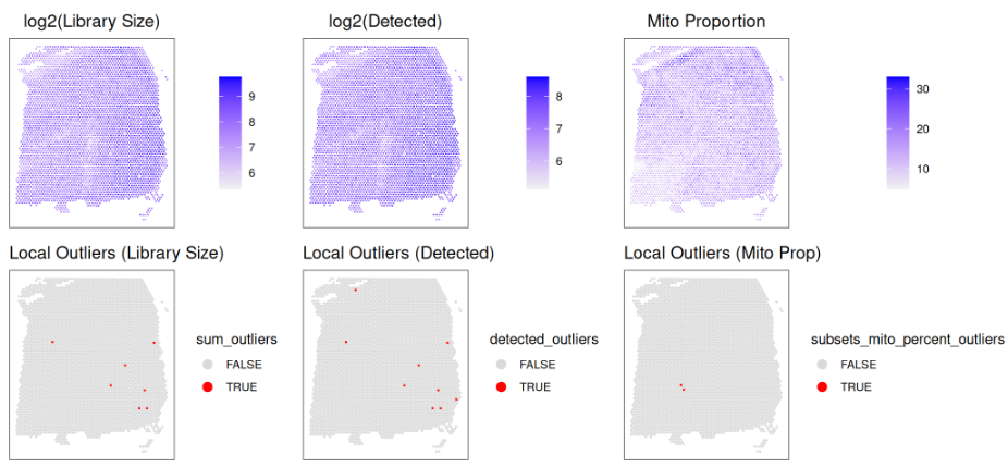
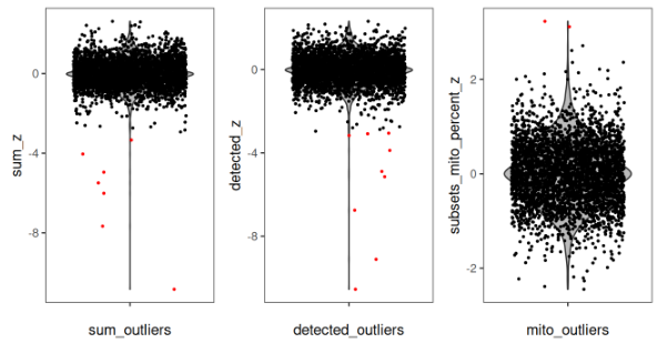
在对数转换后的文库大小和检测到的基因数上尤其明显，在组织区域的右下角存在清晰的异常值。我们还可以看到，这些异常 spot 在底部一行被成功识别。这种“目测检验”是一个良好的诊断方法，用于确认局部异常值被准确检测。另一种做法是，通过小提琴图对每个 spot 的 z-score 转换后的指标进行可视化，从而展示被检测为异常值的 spot。

# z-transformed library size and outliers
p1 <- 
  plotObsQC(spe, plot_type = "violin", x_metric = "sum_z", 
            annotate = "sum_outliers", point_size = 0.5) + 
  xlab("sum_outliers")

# z-transformed detected genes and outliers
p2 <- 
  plotObsQC(spe, plot_type = "violin", x_metric = "detected_z", 
            annotate = "detected_outliers", point_size = 0.5) + 
  xlab("detected_outliers")

# z-transformed mito percent and outliers
p3 <- 
  plotObsQC(spe, plot_type = "violin", x_metric = "subsets_mito_percent_z", 
            annotate = "subsets_mito_percent_outliers", point_size = 0.5) + 
  xlab("mito_outliers")

# plot using patchwork
p1 | p2 | p3