🤩 Seurat | 空间转录组数据分析的标准流程!~(五)(Visium HD与 scRNA-seq反卷积)

🤩 Seurat | 空间转录组数据分析的标准流程!~(五)(Visium HD与 scRNA-seq反卷积)

生信漫卷
发布于 2025-11-13 18:29:39
发布于 2025-11-13 18:29:39
写在前面
哎~ 😞
人生真的是很难呢!~☹️
用到的包
rm(list = ls())
library(Seurat)
library(ggplot2)
library(patchwork)
library(dplyr)
if (!requireNamespace("spacexr", quietly = TRUE)) {
  devtools::install_github("dmcable/spacexr", build_vignettes = FALSE)
}
library(spacexr)
示例数据
localdir <- "./visium_hd/mouse_brain/"
cortex <- Load10X_Spatial(data.dir = localdir, bin.size = c(8, 16))
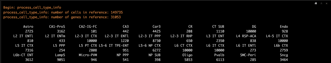
参考单细胞数据!~🫢
# load in the reference scRNA-seq dataset
ref <- readRDS("./allen_scRNAseq_ref.Rds")
NormalizeData
DefaultAssay(cortex) <- "Spatial.008um"
cortex <- NormalizeData(cortex)
无监督聚类
使用Sketch采样,这里我只选了5000细胞。👇
cortex <- FindVariableFeatures(cortex)
cortex <- SketchData(
  object = cortex,
  ncells = 5000,
  method = "LeverageScore",
  sketched.assay = "sketch"
)

DefaultAssay(cortex) <- "sketch"
cortex <- ScaleData(cortex)
cortex <- RunPCA(cortex, assay = "sketch", reduction.name = "pca.cortex.sketch", verbose = T)
cortex <- FindNeighbors(cortex, reduction = "pca.cortex.sketch", dims = 1:50)
cortex <- RunUMAP(cortex, reduction = "pca.cortex.sketch", reduction.name = "umap.cortex.sketch", return.model = T, dims = 1:50, verbose = T)
反卷积
整理参考数据集!~🥳
ref!~
Idents(ref) <- "subclass_label"
counts <- ref[["RNA"]]$counts
cluster <- as.factor(ref$subclass_label)
nUMI <- ref$nCount_RNA
levels(cluster) <- gsub("/", "-", levels(cluster))
cluster <- droplevels(cluster)
构建RCTD参考集。😍
# create the RCTD reference object
reference <- Reference(counts, cluster, nUMI)

counts_hd <- cortex[["sketch"]]$counts
cortex_cells_hd <- colnames(cortex[["sketch"]])
coords <- GetTissueCoordinates(cortex)[cortex_cells_hd, 1:2]

# create the RCTD query object
query <- SpatialRNA(coords, counts_hd, colSums(counts_hd))
开始反卷积!~😂
# run RCTD
RCTD <- create.RCTD(query, reference, max_cores = 6 )
RCTD <- run.RCTD(RCTD, doublet_mode = "doublet")
# add results back to Seurat object
cortex <- AddMetaData(cortex, metadata = RCTD@results$results_df)
投影label!~🫢
# project RCTD labels from sketched cortical cells to all cortical cells
cortex$first_type <- as.character(cortex$first_type)
cortex$first_type[is.na(cortex$first_type)] <- "Unknown"
cortex <- ProjectData(
  object = cortex,
  assay = "Spatial.008um",
  full.reduction = "pca.cortex",
  sketched.assay = "sketch",
  sketched.reduction = "pca.cortex.sketch",
  umap.model = "umap.cortex.sketch",
  dims = 1:50,
  refdata = list(full_first_type = "first_type")
)
DefaultAssay(cortex) <- "Spatial.008um"

# we only ran RCTD on the cortical cells
# set labels to all other cells as "Unknown"
cortex[[]][, "full_first_type"] <- "Unknown"
cortex$full_first_type[Cells(cortex)] <- cortex$full_first_type[Cells(cortex)]
Idents(cortex) <- "full_first_type"

# now we can spatially map the location of any scRNA-seq cell type
# start with Layered (starts with L), excitatory neurons in the cortex
cells <- CellsByIdentities(cortex)
excitatory_names <- sort(grep("^L.* CTX", names(cells), value = TRUE))
p <- SpatialDimPlot(cortex, cells.highlight = cells[excitatory_names], cols.highlight = c("#FFFF00", "grey50"), facet.highlight = T, combine = T, ncol = 4)
p
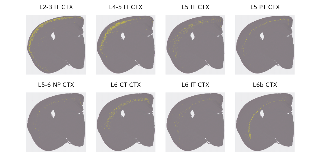
现在可以寻找单个bin的scRNA-seq的Label与组织结构域identity(BANKSY法)之间的关联。🥸
这里我们可以看到兴奋性神经元细胞属于哪些结构域,我们可以将BANKSY聚类重命名为神经元层。😍
plot_cell_types <- function(data, label) {
  p <- ggplot(data, aes(x = get(label), y = n, fill = full_first_type)) +
    geom_bar(stat = "identity", position = "stack") +
    geom_text(aes(label = ifelse(n >= min_count_to_show_label, full_first_type, "")), position = position_stack(vjust = 0.5), size = 2) +
    xlab(label) +
    ylab("# of Spots") +
    ggtitle(paste0("Distribution of Cell Types across ", label)) +
    theme_minimal()
}

cell_type_banksy_counts <- cortex[[]] %>%
  dplyr::filter(full_first_type %in% excitatory_names) %>%
  dplyr::count(full_first_type, banksy_cluster)

min_count_to_show_label <- 20

p <- plot_cell_types(cell_type_banksy_counts, "banksy_cluster")
p
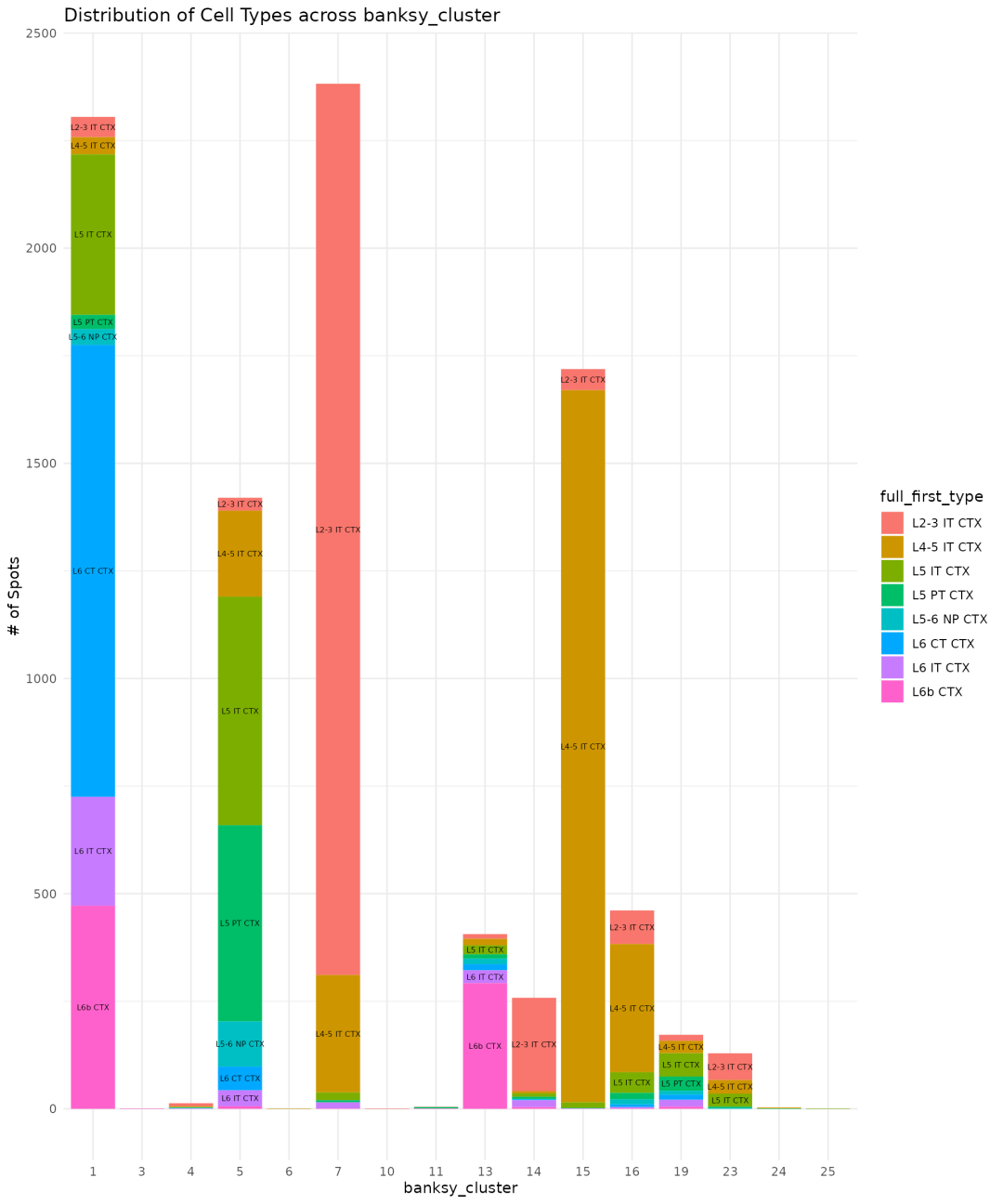
Idents(cortex) <- "banksy_cluster"

cortex$layer_id[WhichCells(cortex, idents = c(7))] <- "Layer 2/3"
cortex$layer_id[WhichCells(cortex, idents = c(15))] <- "Layer 4"
cortex$layer_id[WhichCells(cortex, idents = c(5))] <- "Layer 5"
cortex$layer_id[WhichCells(cortex, idents = c(1))] <- "Layer 6"
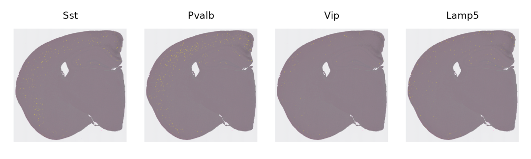
最后,我们可以可视化其他细胞类型的空间分布,看看它们属于哪些皮质层。😏
# set ID to RCTD label
Idents(cortex) <- "full_first_type"

# Visualize distribution of 4 interneuron subtypes
inhibitory_names <- c("Sst", "Pvalb", "Vip", "Lamp5")
cell_ids <- CellsByIdentities(cortex, idents = inhibitory_names)
p <- SpatialDimPlot(cortex, cells.highlight = cell_ids, cols.highlight = c("#FFFF00", "grey50"), facet.highlight = T, combine = T, ncol = 4)
p
可视化细胞类型比例!~🐶
# create barplot to show proportions of cell types of interest
layer_table <- table(cortex$full_first_type, cortex$layer_id)[inhibitory_names, 1:4]

neuron_props <- reshape2::melt(prop.table(layer_table), margin = 1)
ggplot(neuron_props, aes(x = Var1, y = value, fill = Var2)) +
  geom_bar(stat = "identity", position = "fill") +
  labs(x = "Cell type", y = "Proportion", fill = "Layer") +
  theme_classic()

本文参与 腾讯云自媒体同步曝光计划,分享自微信公众号。
原始发表:2025-10-09,如有侵权请联系 cloudcommunity@tencent.com 删除
评论
登录后参与评论
推荐阅读
目录
腾讯云开发者

Copyright © 2013 - 2026 Tencent Cloud. All Rights Reserved. 腾讯云 版权所有
深圳市腾讯计算机系统有限公司 ICP备案/许可证号:粤B2-20090059 ![]() 粤公网安备44030502008569号
粤公网安备44030502008569号
腾讯云计算(北京)有限责任公司 京ICP证150476号 | 京ICP备11018762号