【免疫组库分析】Alakazam包【基因使用、多样性及氨基酸理化性质分析】使用说明

【免疫组库分析】Alakazam包【基因使用、多样性及氨基酸理化性质分析】使用说明

三兔测序学社
发布于 2025-11-20 11:37:35
发布于 2025-11-20 11:37:35
Alakazam基本概况
Alakazam 是适应性免疫受体库测序(AIRR-seq)的 Immcantation 分析框架的一部分,用于研究淋巴细胞受体克隆系谱系、多样性、基因使用情况以及其他库级属性,重点关注高通量免疫球蛋白(Ig)测序。 Alakazam 有五个主要用途: 1.为 Immcantation 框架中的其他 R 包提供核心功能。这包括常见的任务,如文件输入/输出、基本 DNA 序列操作以及与 V(D)J 片段和基因注释的交互。 2.提供与 pRESTO 和 Change-O 工具套件输出交互的 R 接口。 3.对淋巴细胞库进行克隆丰度和多样性分析。 4.对免疫球蛋白序列的克隆群体进行系谱重建,并分析生成的系谱树的拓扑结构。 5.对淋巴细胞受体序列进行理化性质分析。
下载与安装
下载最新稳定版 alakazam 可从 CRAN 或 GitHub 下载。说明:https://alakazam.readthedocs.io/en/stable/vignettes/Diversity-Vignette/
#通过
CRAN 安装最简单:
install.packages("alakazam")
#从
GitHub 下载的源码包可按常规方式安装:
install.packages("alakazam_x.y.z.tar.gz", repos = NULL, type = "source")
# 若安装遇到问题,可能是 Bioconductor 依赖包未满足。可通过以下命令查看所需依赖:
available.packages()["alakazam", "Imports"]
#或使用
Bioconductor 的安装函数:
install.packages("BiocManager")
BiocManager::install("alakazam")
功能描述
文件输入输出
readChangeoDb:输入 Change-O 格式文件。
writeChangeoDb:输出 Change-O 格式文件。
序列清洗
maskSeqEnds:屏蔽序列两端不规则部分。
maskSeqGaps:屏蔽序列中的间隔字符(如 -)。
collapseDuplicates:移除重复序列。
谱系重建
makeChangeoClone:为谱系重建准备序列。
buildPhylipLineage:对 Ig 序列进行谱系重建。
谱系拓扑分析
tableEdges:统计谱系边上的注释关系。
testEdges:对谱系树进行显著性检验。
testMRCA:对最近共同祖先(MRCA)注释进行显著性检验。
summarizeSubtrees:计算谱系子树的多种统计指标。
plotSubtrees:绘制谱系子树的统计指标分布图。
多样性分析
countClones:计算克隆丰度。
estimateAbundance:通过重采样估计克隆丰度曲线。
alphaDiversity:生成克隆多样性曲线。
plotAbundanceCurve:绘制克隆大小分布(秩-丰度曲线)。
plotDiversityCurve:绘制克隆多样性曲线。
plotDiversityTest:在指定多样性指数(Hill 指数)下进行检验并绘图。
Ig 与 TCR 序列注释
countGenes:统计 Ig 和 TCR 等位基因、基因及家族使用情况。
extractVRegion:提取 CDR(互补决定区)和 FWR(框架区)子序列。
getAllele:获取 V(D)J 等位基因名称。
getGene:获取 V(D)J 基因名称。
getFamily:获取 V(D)J 家族名称。
junctionAlignment:分析接头(junction)对齐的序列特征。
序列距离计算
seqDist:计算两个序列的距离。
seqEqual:判断两个序列是否等价。
pairwiseDist:计算一组序列的成对距离矩阵。
pairwiseEqual:计算一组序列的成对等价性逻辑矩阵。
氨基酸性质分析
translateDNA:将 DNA 序列翻译为氨基酸序列。
aminoAcidProperties:计算氨基酸序列的多种理化性质。
countPatterns:统计序列中的模式(如特定氨基酸组合)。数据读取与写入操作指南
数据读取 alakazam 包中包含两种格式的示例数据库:
Change-O格式:ExampleDbChangeo
AIRR格式:ExampleDb
如需了解 AIRR 格式的详细说明,请访问 AIRR Community 文档网站。
示例代码
# 设置包内文件路径(为之前提到的示例数据库的简化版本)
changeo_file <- system.file("extdata", "example_changeo.tab.gz", package = "alakazam")
airr_file <- system.file("extdata", "example_airr.tsv.gz", package = "alakazam")
# 读取数据
db_changeo <- alakazam::readChangeoDb(changeo_file)
db_airr <- airr::read_rearrangement(airr_file)分析
分析1:基因使用分析
基因使用分析只需要以下列:v_call,d_call,j_call
加载所需包
library(alakazam)
library(dplyr)
library(scales)
按样本统计 V(D)J 等位基因、基因或家族的使用情况
可以通过 countGenes 函数获得组内 V(D)J 等位基因、基因或家族的相对丰度。为了分析不同样本之间的 V 基因使用差异,我们将设置 gene="v_call"(包含基因数据的列)和 groups="sample_id"(包含分组变量的列)。为了在基因水平上量化丰度,我们设置 mode="gene"
# 在基因水平上量化使用情况
gene <- countGenes(ExampleDb, gene="v_call", groups="sample_id", mode="gene")
head(gene, n=4)
## # A tibble: 4 × 6
##   sample_id locus gene     seq_count locus_count seq_freq
##   <chr>     <chr> <chr>        <int>       <int>    <dbl>
## 1 +7d       IGH   IGHV3-49       698         999    0.699
## 2 -1h       IGH   IGHV3-9         83        1000    0.083
## 3 -1h       IGH   IGHV5-51        60        1000    0.06
## 4 -1h IGH IGHV3-30 58 1000 0.058在结果数据框中,seq_count 列是每个样本组中给定基因的原始序列数量。seq_freq 是给定样本组中每个基因的频率按等位基因(mode="allele")或家族水平(mode="family")量化使用情况
# 按样本量化 V 家族的使用情况
family <- countGenes(ExampleDb, gene="v_call", groups="sample_id", mode="family")
# 按样本量化 V 等位基因的使用情况
allele <- countGenes(ExampleDb, gene="v_call", groups="sample_id", mode="allele")
# 按样本绘制 V 家族的使用情况
g1 <- ggplot(family, aes(x=gene, y=seq_freq)) +
    theme_bw() +
    ggtitle("家族使用情况") +
    theme(axis.text.x=element_text(angle=45, hjust=1, vjust=1)) +
    ylab("库的百分比") +
    xlab("") +
    scale_y_continuous(labels=percent) +
    scale_color_brewer(palette="Set1") +
    geom_point(aes(color=sample_id), size=5, alpha=0.8, position=position_dodge(width = 0.1))
g2<- ggplot(allele, aes(x=gene, y=seq_freq)) +
    theme_bw() +
    ggtitle("等位基因使用情况") +
    theme(axis.text.x=element_text(angle=45, hjust=1, vjust=1)) +
    ylab("库的百分比") +
    xlab("") +
    scale_y_continuous(labels=percent) +
    scale_color_brewer(palette="Set1") +
    geom_point(aes(color=sample_id), size=5, alpha=0.8, position=position_dodge(width = 0.1))
plot(g1,g2)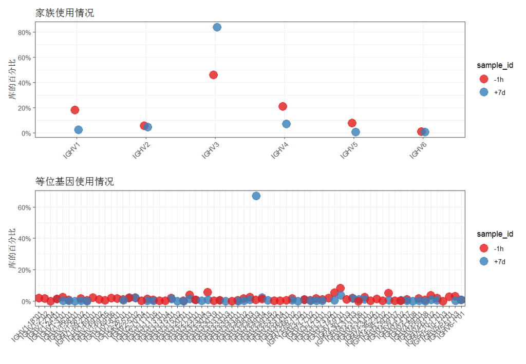
使用额外分组统计基因丰度
countGenes 的 groups 参数可以接受多个分组列,并将在每个唯一组合内计算丰度。在下面的例子中,将按样本和同种型对进行分组(groups=c("sample_id", "c_call"))。此外,我们将通过克隆计数(每个克隆只计数一次,无论该克隆代表多少序列)而不是序列计数来量化丰度。
通过将值传递给 countGenes 的 clone 参数(clone="clone_id")添加克隆标准。对于每个克隆组,只考虑最常见的等位基因/基因/家族进行计数
# 按样本和同种型量化 V 家族的克隆使用情况
family <- countGenes(ExampleDb, gene="v_call", groups=c("sample_id", "c_call"),
                     clone="clone_id", mode="family")
head(family, n=4)
## # A tibble: 4 × 7
##   sample_id c_call locus gene  clone_count locus_clone_count clone_freq
##   <chr>     <chr>  <chr> <chr>       <int>             <int>      <dbl>
## 1 -1h       IGHM   IGH   IGHV3         222               532      0.417
## 2 -1h       IGHM   IGH   IGHV1         110               532      0.207
## 3 -1h       IGHM   IGH   IGHV4         102               532      0.192
## 4 +7d IGHG IGH IGHV3 94 103 0.913数据框包含额外的分组列(c_call),以及 clone_count 和 clone_freq 列,分别代表在给定样本和同种型对中每个 V 家族的克隆计数和频率。# 筛选用于绘图的 IGHM 和 IGHG
family <- filter(family, c_call %in% c("IGHM", "IGHG"))
# 按样本和同种型绘制 V 家族的克隆使用情况
g3 <- ggplot(family, aes(x=gene, y=clone_freq)) +
theme_bw() +
ggtitle("克隆使用情况") +
theme(axis.text.x=element_text(angle=45, hjust=1, vjust=1)) +
ylab("库的百分比") +
xlab("") +
scale_y_continuous(labels=percent) +
scale_color_brewer(palette="Set1") +
geom_point(aes(color=sample_id), size=5, alpha=0.8, position=position_dodge(width = 0.1)) +
facet_grid(. ~ c_call)
plot(g4)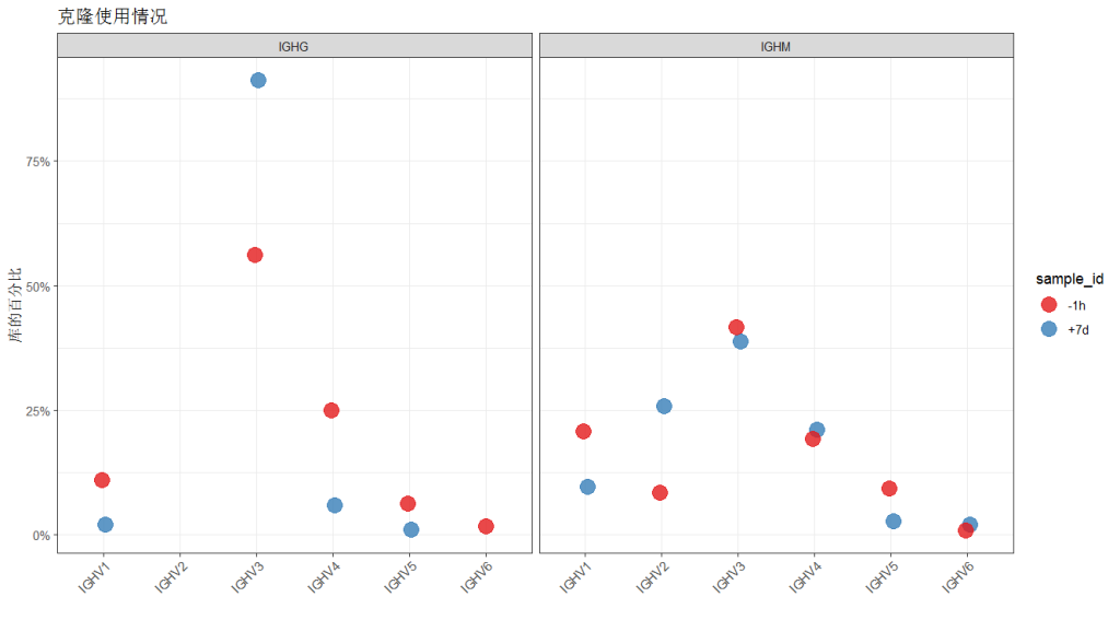
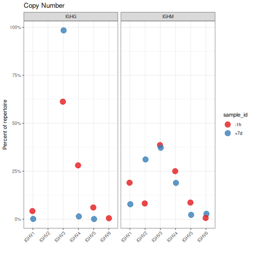
使用序列的拷贝数计算丰度
可以通过序列的拷贝数来计算丰度,而不是通过序列或克隆计数。这可以通过将拷贝数列传递给 copy 参数(copy="duplicate_count")来实现。
在这里需要区分的clone_type与clone_counts的概念,clone_type理解为动物园不同的物种,总数是多少种动物。clone_counts是一个物种的数量,总数是动物数量的总和。因此,这里的duplicated_count是基于Clone_counts来计算的。如果有克隆的扩增会出现许多拷贝数,通过duplicate_count可以发现优势克隆。在基因使用分析中,建个人更倾向于用这个参数(duplicated_count)。如果不关心
# Calculate V family copy numbers by sample and isotype
family <- countGenes(ExampleDb, gene="v_call", groups=c("sample_id", "c_call"),
                     mode="family", copy="duplicate_count")
# Subset to IGHM and IGHG for plotting
family <- filter(family, c_call %in% c("IGHM", "IGHG"))
# Plot V family copy abundance by sample and isotype
g4 <- ggplot(family, aes(x=gene, y=copy_freq)) +
    theme_bw() +
    ggtitle("Copy Number") +
    theme(axis.text.x=element_text(angle=45, hjust=1, vjust=1)) +
    ylab("Percent of repertoire") +
    xlab("") +
    scale_y_continuous(labels=percent) +
    scale_color_brewer(palette="Set1") +
    geom_point(aes(color=sample_id), size=5, alpha=0.8, position=position_dodge(width = 0.1)) +
    facet_grid(. ~ c_call)
plot(g4)
分析2:氨基酸性质分析
可以通过 aminoAcidProperties 函数获取多种氨基酸 理化特征,包括:
length: 氨基酸长度 (total amino acid count) gravy: 平均疏水性 (grand average of hydrophobicity) bulkiness: 平均体积 (average bulkiness) polarity: 平均极性 (average polarity) aliphatic: 归一化脂肪族指数 (normalized aliphatic index) charge: 归一化净电荷 (normalized net charge) acidic: 酸性氨基酸 含量 (acidic side chain residue content) basic: 碱性氨基酸含量 (basic side chain residue content) aromatic: 芳香族氨基酸含量 (aromatic side chain content)
代码举例
# Subset example data
data(ExampleDb)
db <- ExampleDb[ExampleDb$sample_id == "+7d", ]
db_props <- aminoAcidProperties(db, seq="junction", trim=TRUE, label="cdr3")
#
#将DNA序列翻译成氨基酸序列是通过默认的nt
=TRUE参数实现的。
#为了将连接序列减少到CDR3序列
,我们指定了trim=TRUE参数,这将在分析前去除第一个和最后一个密码子(保守的残基)。
#使用label
="cdr3"参数将在输出列名称前添加前缀cdr3
# The full set of properties are calculated by default
dplyr::select(db_props[1:3, ], starts_with("cdr3"))
##   cdr3_aa_length cdr3_aa_gravy cdr3_aa_bulk cdr3_aa_aliphatic cdr3_aa_polarity
## 1             29     0.1724138     14.12345         0.8034483         8.168966
## 2             29    -0.3482759     14.69034         0.6724138         8.255172
## 3             26    -0.9884615     13.96154         0.5653846         8.873077
##   cdr3_aa_charge cdr3_aa_basic cdr3_aa_acidic cdr3_aa_aromatic
## 1     0.03902939     0.1034483     0.06896552       0.06896552
## 2     2.21407038     0.2068966     0.06896552       0.27586207
## 3     1.11045407     0.2307692     0.15384615       0.19230769
可视化分析结果
# Define a ggplot theme for all plots
tmp_theme <- theme_bw() + theme(legend.position="bottom")
# Generate plots for all four of the properties
g1 <- ggplot(db_props, aes(x=c_call, y=cdr3_aa_length)) + tmp_theme +
    ggtitle("CDR3 length") +
    xlab("Isotype") + ylab("Amino acids") +
    scale_fill_manual(name="Isotype", values=IG_COLORS) +
    geom_boxplot(aes(fill=c_call))
g2 <- ggplot(db_props, aes(x=c_call, y=cdr3_aa_gravy)) + tmp_theme +
    ggtitle("CDR3 hydrophobicity") +
    xlab("Isotype") + ylab("GRAVY") +
    scale_fill_manual(name="Isotype", values=IG_COLORS) +
    geom_boxplot(aes(fill=c_call))
g3 <- ggplot(db_props, aes(x=c_call, y=cdr3_aa_basic)) + tmp_theme +
    ggtitle("CDR3 basic residues") +
    xlab("Isotype") + ylab("Basic residues") +
    scale_y_continuous(labels=scales::percent) +
    scale_fill_manual(name="Isotype", values=IG_COLORS) +
    geom_boxplot(aes(fill=c_call))
g4 <- ggplot(db_props, aes(x=c_call, y=cdr3_aa_acidic)) + tmp_theme +
    ggtitle("CDR3 acidic residues") +
    xlab("Isotype") + ylab("Acidic residues") +
    scale_y_continuous(labels=scales::percent) +
    scale_fill_manual(name="Isotype", values=IG_COLORS) +
    geom_boxplot(aes(fill=c_call))
# Plot in a 2x2 grid
gridPlot(g1, g2, g3, g4, ncol=2)
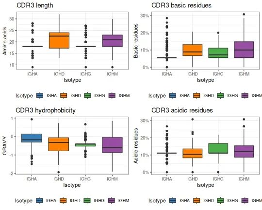
图: CDR3氨基酸理化特征
分析3:多样性分析
这个软件包提供了推断完整克隆丰度分布的方法(使用estimateAbundance函数),以及两种评估这些分布多样性的方法:使用alpha Diversity生成一定多样性阶数(q)范围内的平滑多样性(D)曲线,以及对固定多样性阶数(q)的多样性(D)进行显著性检验。
生成克隆丰度曲线
可以使用countClones函数生成一个克隆丰度计数和频率数据,该函数可以不适用拷贝数(seq_counts,理解为clonetype)或使用拷贝数(copy_count,理解为clonecounts),计算对应频率(seq_freq或者 copy_freq)。
# Partitions the data based on the sample column
clones <- countClones(ExampleDb, group="sample_id")
head(clones, 5)
# Partitions the data based on both the sample_id and c_call columns
# Weights the clone sizes by the duplicate_count column
clones <- countClones(ExampleDb, group=c("sample_id", "c_call"), copy="duplicate_count", clone="clone_id")
head(clones, 5)
#结果如下
## # A tibble: 5 × 7
## # Groups:   sample_id, c_call [2]
##   sample_id c_call clone_id seq_count copy_count seq_freq copy_freq
##   <chr>     <chr>     <dbl>     <int>      <dbl>    <dbl>     <dbl>
## 1 +7d       IGHA       3128        88        651   0.331     0.497
## 2 +7d       IGHG       3100        49        279   0.0928    0.173
## 3 +7d       IGHA       3141        44        240   0.165     0.183
## 4 +7d       IGHG       3192        19        141   0.0360    0.0874
## 5 +7d       IGHG       3177        29        130   0.0549    0.0806
虽然countClones会报告观察到的丰度,但它不会提供置信区间。使用estimateAbundance函数通过自举法推导置信区间来推断完整的克隆丰度分布。可以使用plotAbundanceCurve函数可视化此输出。
# Partitions the data on the sample column
# Calculates a 95% confidence interval via 100 bootstrap realizations 100次重抽样和模型训练的过程
curve <- estimateAbundance(ExampleDb, group="sample_id", ci=0.95, nboot=100, clone="clone_id")
# Plots a rank abundance curve of the relative clonal abundances
sample_colors <- c("-1h"="seagreen", "+7d"="steelblue")
plot(curve, colors = sample_colors, legend_title="Sample")
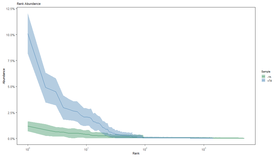
编者理解是每一个克隆频率的累加曲线图。X轴是克隆的排序,按照占比排序。Y轴是对应的累加丰度。
引入思考:丰度与频率的比较
1. 定义与计算方式不同
丰度(Abundance)
定义:指某一类别在总体中的绝对数量或相对比例,通常用于描述连续或离散数据的分布。
计算公式:
绝对丰度:某类别的实际数量(如某元素在样本中的原子数)。
相对丰度:(某类别的数量 / 总数量)× 100%(结果以百分比表示)。
特点:
强调“总量”或“占比”,常用于生态学、化学、基因组学等领域。
例如:土壤中某种细菌的丰度为20%,表示其占总微生物的20%。
频率(Frequency)
定义:指某一事件或类别在重复实验或观测中出现的次数,是概率的基础。
计算公式:
绝对频率:某事件发生的次数(如抛硬币正面朝上10次)。
相对频率:(某事件发生次数 / 总实验次数)× 100%。
特点:
强调“重复观测中的出现概率”,常用于概率统计、实验科学。
例如:抛硬币100次,正面朝上50次,频率为50%。
2. 应用场景不同
丰度的典型场景:
生态学:物种在生态系统中的数量占比。
化学:同位素在元素中的相对含量。
基因组学:基因或序列在样本中的覆盖度。
核心:描述静态分布或组成。
频率的典型场景:
概率统计:事件发生的长期概率(如抛硬币、骰子)。
质量控制:产品缺陷率。
核心:描述动态重复实验中的规律。
3. 为何丰度不是频率?
侧重点不同:
丰度关注“总量中的占比”(如某元素占样本的30%)。
频率关注“重复实验中的出现概率”(如某事件在100次实验中发生30次)。
数据性质不同:
丰度常用于静态数据(如样本成分分析)。
频率常用于动态数据(如实验重复观测)。
数学表达差异:
丰度可以是绝对值或相对值,而频率通常与实验次数直接相关
在此R包中,用丰度来描述克隆在整体免疫组库中的占比,并计算丰度曲线。在许多免疫组库文章中也将丰度与频率混为一谈,因为测序所用的样本也是抽样的结果,免疫状态也是动态结果,其二,更容易被理解。
生成多样性曲线函数alphaDiversity对输入序列进行均匀重采样,并使用每次重采样实现重新计算克隆大小分布和多样性。多样性(D)是根据一系列多样性阶数(q)计算的,以生成平滑的曲线。
qD = (∑piq)1/(1-q)
理解q值的含义
q值是Hill numbers多样性指数族中的一个参数,它决定了多样性计算时对稀有物种和常见物种的权重分配。
当q取不同值时,多样性指数的生物学意义和数学特性会发生变化:
q=0:仅考虑物种丰富度,完全忽略物种的相对丰度,对稀有物种最敏感
q=1:对应Shannon熵的指数形式,平等考虑所有物种
q=2:对应Simpson指数的倒数,对常见物种更敏感
q=3、4:随着q值增大,多样性指数对高丰度物种的权重进一步增加
意义:
覆盖完整的敏感度谱系:能从关注物种存在与否(q=0)到关注优势物种(q=4),全面反映群落多样性。
包含经典多样性指数:q=1时等价于Shannon-Wiener指数,q=2时等价于Simpson多样性指数。
提供充分的比较维度:通过q=1、2、3、4时的多样性曲线变化,可判断群落是由优势种主导还是物种均匀组成。
数学和生物学合理性:q值大于4时,多样性指数对物种分布的敏感性变化平缓,继续增加q值对分析结果提升有限。# Compare diversity curve across values in the "sample" column
# q ranges from 0 (min_q=0) to 4 (max_q=4) in 0.05 increments (step_q=0.05)
# A 95% confidence interval will be calculated (ci=0.95)
# 100 resampling realizations are performed (nboot=100)
sample_curve <- alphaDiversity(ExampleDb, group="sample_id", clone="clone_id",
min_q=0, max_q=4, step_q=0.1,
ci=0.95, nboot=100)
# Plot a log-log (log_q=TRUE, log_d=TRUE) plot of sample diversity
# Indicate number of sequences resampled from each group in the title
sample_main <- paste0("Sample diversity")
sample_colors <- c("-1h"="seagreen", "+7d"="steelblue")
plot(sample_curve, colors=sample_colors, main_title=sample_main,
legend_title="Sample")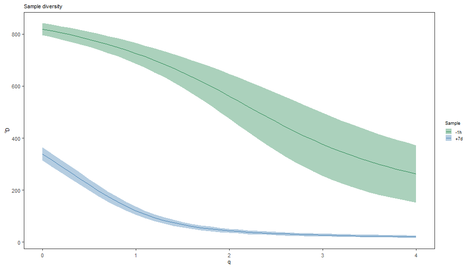
# Compare diversity curve across values in the c_call column
# Analyse is restricted to c_call values with at least 30 sequences by min_n=30
# Excluded groups are indicated by a warning message
isotype_curve <- alphaDiversity(ExampleDb, group="c_call", clone="clone_id",
                                min_q=0, max_q=4, step_q=0.1,
                                ci=0.95, nboot=100)
# Plot isotype diversity using default set of Ig isotype colors
isotype_main <- paste0("Isotype diversity")
plot(isotype_curve, colors=IG_COLORS, main_title=isotype_main,
     legend_title="Isotype")
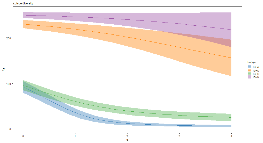
不同IGH亚型多样性指数比较
# Test diversity at q=0, q=1 and q=2 (equivalent to species richness, Shannon entropy,
# Simpson's index) across values in the sample_id column
# 100 bootstrap realizations are performed (nboot=100)
isotype_test <- alphaDiversity(ExampleDb, group="c_call", min_q=0, max_q=2, step_q=1, nboot=100, clone="clone_id")
# Print P-value table
print(isotype_test@tests)
## # A tibble: 18 × 5
##    test         q     delta_mean delta_sd pvalue
##    <chr>        <chr>      <dbl>    <dbl>  <dbl>
##  1 IGHA != IGHD 0         140.       8.07   0
##  2 IGHA != IGHD 1         184.       8.28   0
##  3 IGHA != IGHD 2         190.      11.4    0
##  4 IGHA != IGHG 0           5.09     8.35   0.64
##  5 IGHA != IGHG 1          25.1      5.99   0
##  6 IGHA != IGHG 2          27.1      4.43   0
##  7 IGHA != IGHM 0         160.       6.22   0
##  8 IGHA != IGHM 1         213.       5.52   0
##  9 IGHA != IGHM 2         230.       6.73   0
## 10 IGHD != IGHG 0         135.       8.30   0
## 11 IGHD != IGHG 1         159.       9.21   0
## 12 IGHD != IGHG 2         162.      12.4    0
## 13 IGHD != IGHM 0          20.6      6.48   0
## 14 IGHD != IGHM 1          28.7      9.07   0
## 15 IGHD != IGHM 2          40.7     13.6    0
## 16 IGHG != IGHM 0         155.       6.52   0
## 17 IGHG != IGHM 1         188.       6.23   0
## 18 IGHG != IGHM 2 203. 7.71 # Plot results at q=0 and q=2
# Plot the mean and standard deviations at q=0 and q=2
plot(isotype_test, 0, colors=IG_COLORS, main_title=isotype_main,
legend_title="Isotype")
plot(isotype_test, 2, colors=IG_COLORS, main_title=isotype_main,
legend_title="Isotype")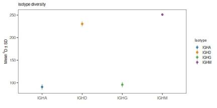
本文参与 腾讯云自媒体同步曝光计划,分享自微信公众号。
原始发表:2025-11-02,如有侵权请联系 cloudcommunity@tencent.com 删除
评论
登录后参与评论
推荐阅读
目录
腾讯云开发者

Copyright © 2013 - 2026 Tencent Cloud. All Rights Reserved. 腾讯云 版权所有
深圳市腾讯计算机系统有限公司 ICP备案/许可证号:粤B2-20090059 ![]() 粤公网安备44030502008569号
粤公网安备44030502008569号
腾讯云计算(北京)有限责任公司 京ICP证150476号 | 京ICP备11018762号