《数字图像处理》第 4 章 - 频率域滤波

啊阿狸不会拉杆

发布于 2026-01-21 13:46:38

1280

引言

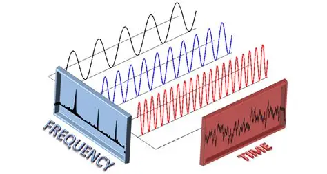
在数字图像处理领域，空间域滤波是我们最开始接触的基础操作，但面对复杂的图像增强、去噪等需求时，频率域滤波往往能展现出更强大的优势。频率域的核心思想是将图像从空间域转换到频率域，对不同频率分量进行针对性处理后，再转换回空间域得到处理结果。

简单来说，图像中的低频分量对应着图像的整体轮廓、大的结构，而高频分量对应着边缘、细节、噪声等。频率域滤波就是通过设计滤波器，保留或抑制特定频率分量，从而实现图像的平滑、锐化、去噪等目标。本章将从基础概念到实战应用，全方位拆解频率域滤波的知识体系，让你从零掌握这一核心技术。

学习目标

理解傅里叶变换的核心原理，掌握连续 / 离散、单变量 / 二变量傅里叶变换的推导与应用；
掌握取样、混叠、取样定理等关键概念，理解其对数字图像傅里叶变换的影响；
熟悉二维 DFT 的核心性质，能运用这些性质解决实际处理问题；
掌握频率域滤波的基本流程，能独立设计低通、高通、选择性滤波器；
能够使用 Python 实现各类频率域滤波算法，并分析不同滤波器的效果差异；
理解 FFT 的原理与优势，掌握其在图像频率域处理中的高效应用。

4.1 背景

4.1.1 傅里叶级数和变换简史

傅里叶的核心思想最早由法国数学家约瑟夫・傅里叶于 19 世纪初提出，他在研究热传导问题时发现：任何周期函数都可以表示为不同频率的正弦 / 余弦函数的线性组合（傅里叶级数）。这一思想后来被拓展到非周期函数，形成了傅里叶变换 —— 将非周期函数分解为连续的频率分量。

在数字图像处理领域，傅里叶变换的离散化（DFT）是关键里程碑，而快速傅里叶变换（FFT）的出现则解决了 DFT 计算复杂度高的问题，让频率域处理从理论走向实际应用。

4.1.2 关于本章中的例子

本章所有示例均基于 Python 实现，使用numpy处理数值计算、matplotlib可视化、cv2读取 / 处理图像。所有代码均可直接运行，运行前确保安装依赖：

pip install numpy matplotlib opencv-python

4.2 基本概念

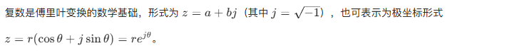
4.2.1 复数

Python 示例：复数基本操作

import numpy as np

# 定义复数
z1 = 3 + 4j
z2 = 1 - 2j

# 复数运算
z_add = z1 + z2  # 加法
z_mul = z1 * z2  # 乘法
z_abs = np.abs(z1)  # 模长
z_angle = np.angle(z1)  # 辐角（弧度）
z_conj = np.conj(z1)  # 共轭复数

# 输出结果
print(f"复数z1: {z1}")
print(f"z1+z2: {z_add}")
print(f"z1*z2: {z_mul}")
print(f"z1模长: {z_abs}, 辐角: {z_angle:.2f}弧度")
print(f"z1共轭: {z_conj}")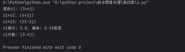

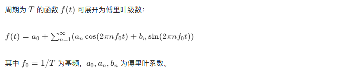
4.2.2 傅里叶级数

Python 示例：傅里叶级数逼近方波

import numpy as np
import matplotlib.pyplot as plt

# 设置中文字体
plt.rcParams["font.sans-serif"] = ["SimHei"]  # 显示中文
plt.rcParams["axes.unicode_minus"] = False    # 显示负号

# 生成时间序列
t = np.linspace(-2*np.pi, 2*np.pi, 1000)

# 方波函数（周期2π）
def square_wave(t):
    return np.where(np.mod(t, 2*np.pi) < np.pi, 1, -1)

# 傅里叶级数逼近
def fourier_series_square(t, n_terms):
    """
    n_terms: 傅里叶级数项数
    """
    result = 0
    for n in range(1, n_terms+1, 2):  # 方波只有奇次谐波
        result += (4/(np.pi*n)) * np.sin(n*t)
    return result

# 计算不同项数的逼近结果
y_original = square_wave(t)
y_5 = fourier_series_square(t, 5)
y_15 = fourier_series_square(t, 15)
y_50 = fourier_series_square(t, 50)

# 绘图对比
fig, axes = plt.subplots(2, 2, figsize=(12, 8))
axes[0,0].plot(t, y_original, label="原始方波", color="red")
axes[0,0].plot(t, y_5, label="5项级数", linestyle="--")
axes[0,0].set_title("5项傅里叶级数逼近")
axes[0,0].legend()
axes[0,0].grid(True)

axes[0,1].plot(t, y_original, label="原始方波", color="red")
axes[0,1].plot(t, y_15, label="15项级数", linestyle="--")
axes[0,1].set_title("15项傅里叶级数逼近")
axes[0,1].legend()
axes[0,1].grid(True)

axes[1,0].plot(t, y_original, label="原始方波", color="red")
axes[1,0].plot(t, y_50, label="50项级数", linestyle="--")
axes[1,0].set_title("50项傅里叶级数逼近")
axes[1,0].legend()
axes[1,0].grid(True)

axes[1,1].plot(t, y_original, label="原始方波", color="red")
axes[1,1].set_title("原始方波")
axes[1,1].legend()
axes[1,1].grid(True)

plt.tight_layout()
plt.show()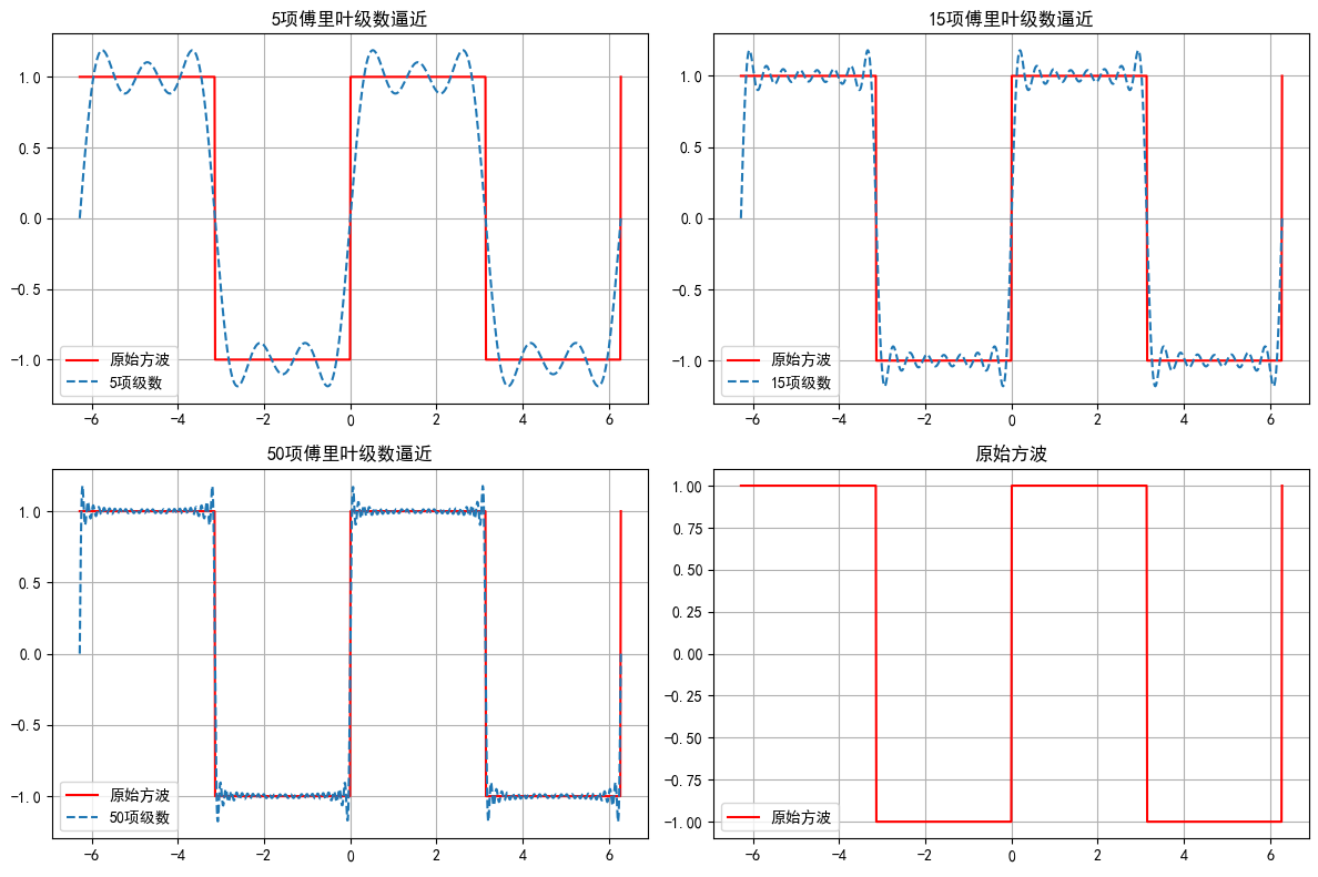

效果说明：项数越多，傅里叶级数越接近原始方波，直观体现了 “不同频率正弦波叠加可逼近周期函数” 的核心思想。

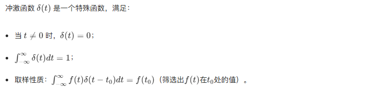
4.2.3 冲激函数及其取样（筛选）性质

Python 示例：冲激函数取样性质模拟

import numpy as np
import matplotlib.pyplot as plt

plt.rcParams["font.sans-serif"] = ["SimHei"]
plt.rcParams["axes.unicode_minus"] = False

# 模拟冲激函数（离散近似）
def delta(t, t0, eps=1e-2):
    """离散近似冲激函数"""
    return np.where(np.abs(t - t0) < eps, 1/eps, 0)

# 定义测试函数
def f(t):
    return np.sin(t) + 0.5*np.cos(2*t)

# 生成时间序列
t = np.linspace(-np.pi, np.pi, 1000)
t0 = np.pi/4  # 取样点
dt = t[1] - t[0]

# 计算f(t)*δ(t-t0)
delta_t = delta(t, t0)
f_delta = f(t) * delta_t

# 积分（离散求和）
sampled_value = np.sum(f_delta) * dt

# 绘图
fig, axes = plt.subplots(2, 1, figsize=(10, 6))
axes[0].plot(t, f(t), label="f(t) = sin(t) + 0.5cos(2t)")
axes[0].scatter(t0, f(t0), color="red", s=100, label=f"取样点 t0={t0:.2f}")
axes[0].set_title("原始函数与取样点")
axes[0].legend()
axes[0].grid(True)

axes[1].plot(t, f_delta, label="f(t)*δ(t-t0)")
axes[1].fill_between(t, 0, f_delta, alpha=0.3, color="orange")
axes[1].set_title(f"f(t)*δ(t-t0) 积分结果：{sampled_value:.4f}（理论值：{f(t0):.4f}）")
axes[1].legend()
axes[1].grid(True)

plt.tight_layout()
plt.show()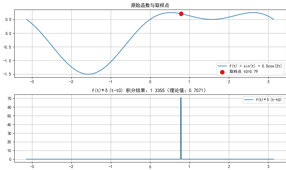

效果说明：积分结果与f(t0)几乎一致，验证了冲激函数的取样性质。

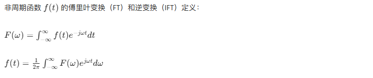
4.2.4 连续单变量函数的傅里叶变换

4.2.5 卷积

Python 示例：卷积定理验证（连续近似）

import numpy as np
import matplotlib.pyplot as plt
from scipy.signal import convolve

plt.rcParams["font.sans-serif"] = ["SimHei"]
plt.rcParams["axes.unicode_minus"] = False

# 定义两个测试函数
t = np.linspace(-5, 5, 1000)
dt = t[1] - t[0]
f = np.exp(-t**2)  # 高斯函数
g = np.where(np.abs(t) < 1, 1, 0)  # 矩形窗

# 方法1：空间域卷积
conv_spatial = convolve(f, g, mode="same") * dt

# 方法2：频率域乘积（FFT）
f_fft = np.fft.fft(f)
g_fft = np.fft.fft(g)
conv_freq = np.fft.ifft(f_fft * g_fft).real * dt

# 绘图对比
fig, axes = plt.subplots(3, 1, figsize=(10, 8))
axes[0].plot(t, f, label="f(t) 高斯函数")
axes[0].plot(t, g, label="g(t) 矩形窗", alpha=0.7)
axes[0].set_title("原始函数")
axes[0].legend()
axes[0].grid(True)

axes[1].plot(t, conv_spatial, label="空间域卷积结果", color="red")
axes[1].set_title("空间域卷积")
axes[1].legend()
axes[1].grid(True)

axes[2].plot(t, conv_freq, label="频率域乘积逆变换结果", color="blue")
axes[2].set_title("频率域处理（卷积定理）")
axes[2].legend()
axes[2].grid(True)

plt.tight_layout()
plt.show()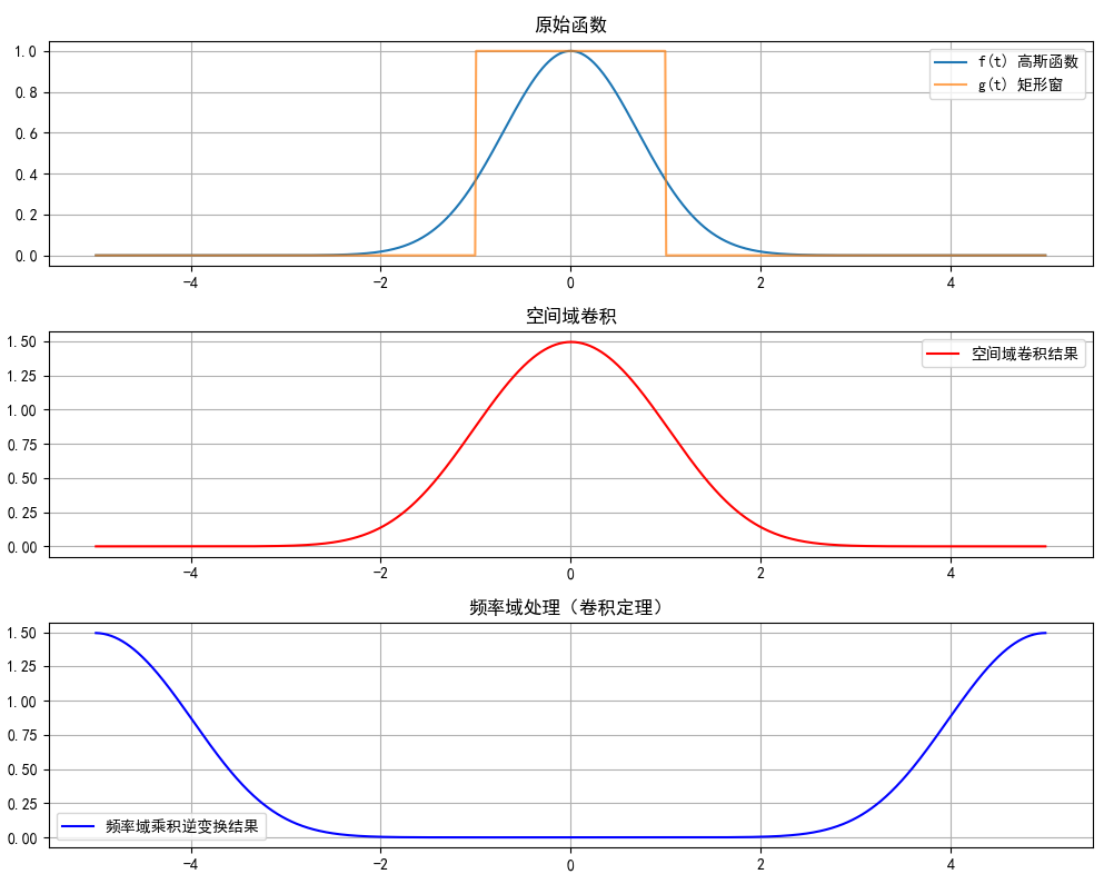

效果说明：两种方法结果几乎完全一致，验证了卷积定理 —— 空间域卷积等价于频率域乘积。

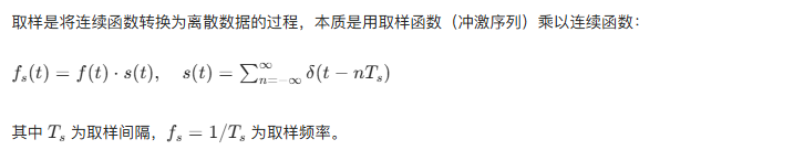
4.3 取样和取样函数的傅里叶变换

4.3.1 取样

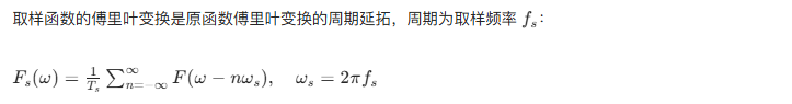
4.3.2 取样后的函数的傅里叶变换

4.3.3 取样定理

为避免混叠，取样频率必须大于信号最高频率的 2 倍：fs>2fmax（奈奎斯特频率）。

4.3.4 混叠

当取样频率不满足取样定理时，周期延拓的频谱会重叠，导致离散信号无法恢复原始连续信号，这种现象称为混叠。

Python 示例：取样与混叠效果对比

import numpy as np
import matplotlib.pyplot as plt
from scipy.interpolate import interp1d

# 设置中文字体
plt.rcParams["font.sans-serif"] = ["SimHei"]
plt.rcParams["axes.unicode_minus"] = False

# 定义原始连续信号（最高频率5Hz）
f_max = 5
t_continuous = np.linspace(0, 2, 1000)
x_continuous = np.sin(2*np.pi*f_max*t_continuous) + 0.5*np.sin(2*np.pi*2*t_continuous)

# 两种取样频率
f_s1 = 15  # 满足取样定理（15>2*5）
f_s2 = 8   # 不满足取样定理（8<2*5）

# 修复：生成取样点时确保包含终点2，避免插值越界
# 使用np.linspace替代np.arange，精准控制取样点范围和数量
n1 = int(f_s1 * 2)  # 2秒内的取样点数
n2 = int(f_s2 * 2)
t1 = np.linspace(0, 2, n1, endpoint=True)  # 包含终点2
t2 = np.linspace(0, 2, n2, endpoint=True)

# 计算取样点的信号值
x1 = np.sin(2*np.pi*f_max*t1) + 0.5*np.sin(2*np.pi*2*t1)
x2 = np.sin(2*np.pi*f_max*t2) + 0.5*np.sin(2*np.pi*2*t2)

# 插值恢复（增加fill_value参数，处理可能的边界微小误差）
interp1 = interp1d(t1, x1, kind="cubic", fill_value="extrapolate")  # 外推边界
interp2 = interp1d(t2, x2, kind="cubic", fill_value="extrapolate")
x_recon1 = interp1(t_continuous)
x_recon2 = interp2(t_continuous)

# 绘图
fig, axes = plt.subplots(2, 1, figsize=(10, 8))

# 子图1：满足取样定理（无混叠）
axes[0].plot(t_continuous, x_continuous, label="原始连续信号", color="blue", linewidth=1.5)
axes[0].scatter(t1, x1, color="red", s=50, label=f"取样点 (fs={f_s1}Hz)")
axes[0].plot(t_continuous, x_recon1, linestyle="--", color="orange", label="恢复信号", linewidth=2)
axes[0].set_title("满足取样定理（无混叠）", fontsize=12)
axes[0].legend(fontsize=10)
axes[0].grid(True, alpha=0.3)
axes[0].set_xlabel("时间 (s)", fontsize=10)
axes[0].set_ylabel("信号幅值", fontsize=10)

# 子图2：不满足取样定理（混叠）
axes[1].plot(t_continuous, x_continuous, label="原始连续信号", color="blue", linewidth=1.5)
axes[1].scatter(t2, x2, color="red", s=50, label=f"取样点 (fs={f_s2}Hz)")
axes[1].plot(t_continuous, x_recon2, linestyle="--", color="orange", label="恢复信号", linewidth=2)
axes[1].set_title("不满足取样定理（混叠）", fontsize=12)
axes[1].legend(fontsize=10)
axes[1].grid(True, alpha=0.3)
axes[1].set_xlabel("时间 (s)", fontsize=10)
axes[1].set_ylabel("信号幅值", fontsize=10)

plt.tight_layout()
plt.show()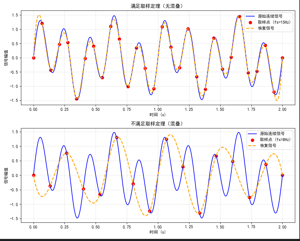

效果说明：满足取样定理时，恢复信号与原始信号几乎一致；不满足时，恢复信号出现明显失真（混叠）。

4.3.5 由取样后的数据重建（复原）函数

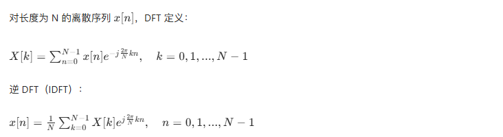
4.4 单变量的离散傅里叶变换

4.4.1 由取样后的函数的连续变换得到 DFT

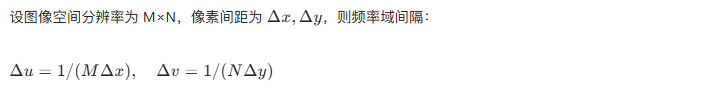
4.4.2 取样和频率间隔的关系

4.5 二变量函数的傅里叶变换

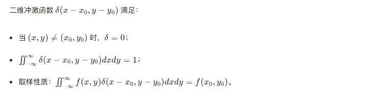
4.5.1 二维冲激及其取样性质

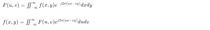
4.5.2 二维连续傅里叶变换对

4.5.3 二维取样和二维取样定理

4.5.4 图像中的混叠

图像是二维信号，取样不足（分辨率过低）会导致混叠，表现为图像边缘模糊、出现摩尔纹等。

4.5.5 二维离散傅里叶变换及其反变换

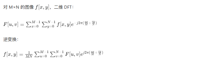
Python 示例：图像的二维 DFT 与 IDFT

import numpy as np
import cv2
import matplotlib.pyplot as plt

plt.rcParams["font.sans-serif"] = ["SimHei"]
plt.rcParams["axes.unicode_minus"] = False

# 读取图像（灰度图）
img = cv2.imread("lena.jpg", 0)  # 替换为你的图像路径，若无lena图可生成测试图
if img is None:
    # 生成测试图（棋盘格）
    img = np.zeros((256, 256), dtype=np.uint8)
    img[::16, ::16] = 255
    img[8::16, 8::16] = 255

# 二维DFT（FFT加速）
dft = np.fft.fft2(img)
dft_shift = np.fft.fftshift(dft)  # 零频率移到中心

# 傅里叶频谱（对数缩放便于显示）
magnitude_spectrum = 20 * np.log(np.abs(dft_shift) + 1e-8)

# IDFT
idft_shift = np.fft.ifftshift(dft_shift)
img_recon = np.fft.ifft2(idft_shift).real

# 绘图
fig, axes = plt.subplots(1, 3, figsize=(15, 5))
axes[0].imshow(img, cmap="gray")
axes[0].set_title("原始图像")
axes[0].axis("off")

axes[1].imshow(magnitude_spectrum, cmap="gray")
axes[1].set_title("傅里叶频谱（中心化）")
axes[1].axis("off")

axes[2].imshow(img_recon, cmap="gray")
axes[2].set_title("IDFT恢复图像")
axes[2].axis("off")

plt.tight_layout()
plt.show()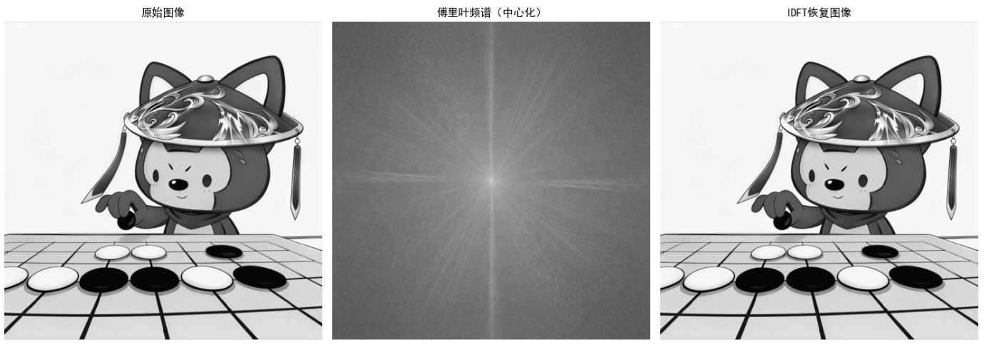

效果说明：恢复图像与原始图像几乎一致，验证了二维 DFT/IDFT 的正确性；频谱图中，中心为低频（亮），边缘为高频（暗）。

4.6 二维 DFT 和 IDFT 的一些性质

4.6.1 空间间隔和频率间隔的关系

4.6.2 平移和旋转

Python 示例：图像平移与旋转的 DFT 效果

import numpy as np
import cv2
import matplotlib.pyplot as plt

plt.rcParams["font.sans-serif"] = ["SimHei"]
plt.rcParams["axes.unicode_minus"] = False

# 生成测试图像（中心矩形）
img = np.zeros((256, 256), dtype=np.uint8)
img[100:156, 100:156] = 255

# 1. 平移效果
M_trans = np.float32([[1,0,30],[0,1,30]])
img_trans = cv2.warpAffine(img, M_trans, (256,256))

# 2. 旋转效果
rows, cols = img.shape
M_rot = cv2.getRotationMatrix2D((cols/2, rows/2), 45, 1)
img_rot = cv2.warpAffine(img, M_rot, (cols, rows))

# 计算DFT并中心化
def dft_center(img):
    dft = np.fft.fft2(img)
    dft_shift = np.fft.fftshift(dft)
    return 20 * np.log(np.abs(dft_shift) + 1e-8)

spec_original = dft_center(img)
spec_trans = dft_center(img_trans)
spec_rot = dft_center(img_rot)

# 绘图
fig, axes = plt.subplots(2, 3, figsize=(15, 10))
# 空间域
axes[0,0].imshow(img, cmap="gray")
axes[0,0].set_title("原始图像")
axes[0,0].axis("off")
axes[0,1].imshow(img_trans, cmap="gray")
axes[0,1].set_title("平移图像")
axes[0,1].axis("off")
axes[0,2].imshow(img_rot, cmap="gray")
axes[0,2].set_title("旋转45°图像")
axes[0,2].axis("off")

# 频率域
axes[1,0].imshow(spec_original, cmap="gray")
axes[1,0].set_title("原始频谱")
axes[1,0].axis("off")
axes[1,1].imshow(spec_trans, cmap="gray")
axes[1,1].set_title("平移后频谱")
axes[1,1].axis("off")
axes[1,2].imshow(spec_rot, cmap="gray")
axes[1,2].set_title("旋转后频谱")
axes[1,2].axis("off")

plt.tight_layout()
plt.show()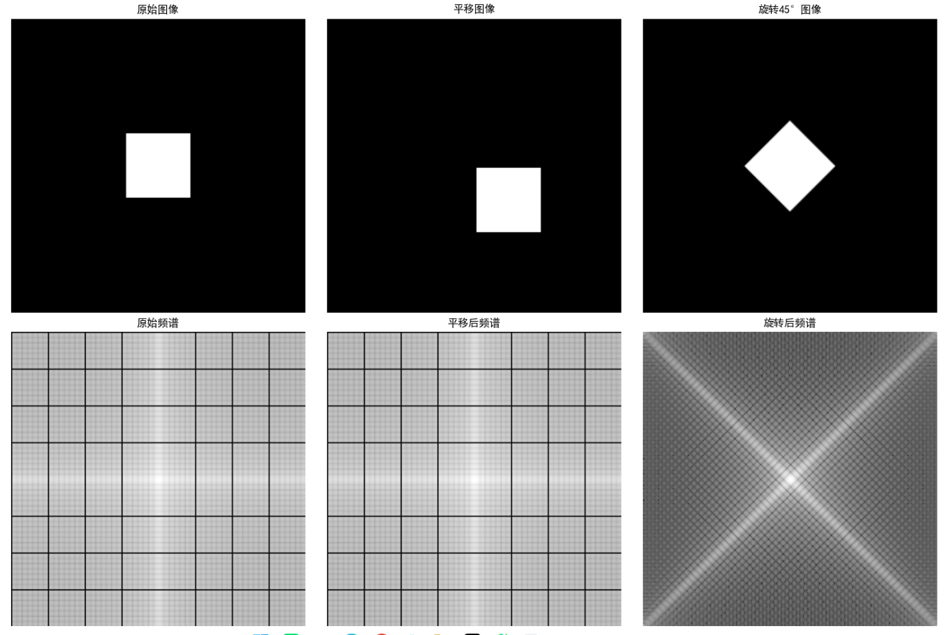

效果说明：平移后的频谱幅值无变化（仅相位变化），旋转后的频谱同步旋转 45°。

4.6.3 周期性

4.6.4 对称性

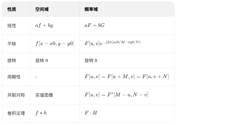
实值图像的 DFT 满足共轭对称性：F[u,v]=F∗[M−u,N−v]，因此频谱关于中心对称。

4.6.5 傅里叶频谱和相角

DFT 结果可分解为幅值（频谱）和相位：F[u,v]=∣F[u,v]∣ejϕ(u,v)其中 ∣F[u,v]∣ 为频谱，ϕ(u,v) 为相角。

Python 示例：频谱与相角可视化

import numpy as np
import cv2
import matplotlib.pyplot as plt

plt.rcParams["font.sans-serif"] = ["SimHei"]
plt.rcParams["axes.unicode_minus"] = False

# 读取图像
img = cv2.imread("lena.jpg", 0)
if img is None:
    img = np.random.randint(0, 255, (256, 256), dtype=np.uint8)

# DFT
dft = np.fft.fft2(img)
dft_shift = np.fft.fftshift(dft)

# 频谱和相角
magnitude = 20 * np.log(np.abs(dft_shift) + 1e-8)
phase = np.angle(dft_shift)

# 绘图
fig, axes = plt.subplots(1, 3, figsize=(15, 5))
axes[0].imshow(img, cmap="gray")
axes[0].set_title("原始图像")
axes[0].axis("off")

axes[1].imshow(magnitude, cmap="gray")
axes[1].set_title("傅里叶频谱（对数缩放）")
axes[1].axis("off")

axes[2].imshow(phase, cmap="hsv")  # HSV色板更易区分相位
axes[2].set_title("相角")
axes[2].axis("off")

plt.tight_layout()
plt.show()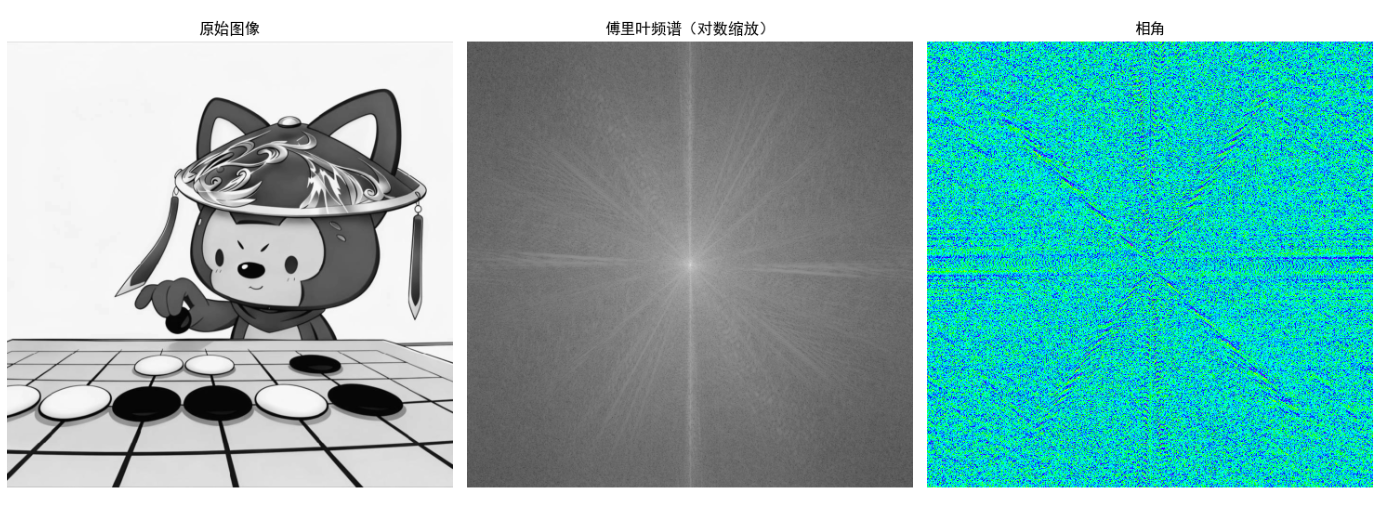

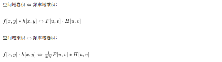
4.6.6 二维离散卷积定理

4.6.7 二维离散傅里叶变换性质的小结

4.7 频率域滤波基础

4.7.1 频率域的其他特性

低频分量：对应图像慢变化的灰度（如背景、大轮廓）；
高频分量：对应图像快变化的灰度（如边缘、细节、噪声）；
滤波核心：通过滤波器 H[u,v] 调整 F[u,v] 的频率分量，G[u,v]=F[u,v]⋅H[u,v]。

4.7.2 频率域滤波基础知识

频率域滤波的本质是对图像的频率分量进行选择性修改，核心逻辑是利用傅里叶变换将图像从空间域映射到频率域，通过设计特定的滤波器函数调整不同频率分量的权重，再通过逆傅里叶变换还原到空间域，实现图像增强、去噪、锐化等目标。

4.7.3 频率域滤波步骤小结

预处理：将图像转换为灰度图，必要时补零至合适尺寸（如 2 的幂次，加速 FFT）；
傅里叶变换：计算 DFT 并将零频率移到中心；
滤波器设计：生成与频谱同尺寸的滤波器 H[u,v]；
频率域处理：G[u,v]=F[u,v]⋅H[u,v]；
逆变换：IDFT 转换回空间域，取实部（虚部为数值误差）；
后处理：归一化灰度值至 [0,255]，得到最终图像。

4.7.4 空间域和频率域滤波之间的对应关系

空间域	频率域
平滑（低通）	抑制高频分量
锐化（高通）	抑制低频分量，增强高频分量
线性滤波	卷积操作	乘积操作
模板越小	滤波器越宽（频率域）
模板越大	滤波器越窄（频率域）

4.8 使用低通频率域滤波器平滑图像

低通滤波器（LPF）：保留低频分量，抑制高频分量，实现图像平滑、去噪。

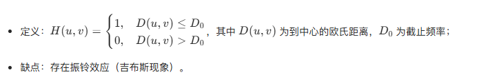
4.8.1 理想低通滤波器（ILPF）

4.8.2 高斯低通滤波器（GLPF）

4.8.3 巴特沃斯低通滤波器（BLPF）

4.8.4 低通滤波的其他例子

Python 示例：三种低通滤波器效果对比

import numpy as np
import cv2
import matplotlib.pyplot as plt

plt.rcParams["font.sans-serif"] = ["SimHei"]
plt.rcParams["axes.unicode_minus"] = False

# 1. 读取并预处理图像
img = cv2.imread("lena.jpg", 0)
if img is None:
    img = np.zeros((256, 256), dtype=np.uint8)
    cv2.circle(img, (128, 128), 60, 255, -1)
    # 添加噪声
    noise = np.random.normal(0, 30, img.shape).astype(np.int16)
    img = np.clip(img + noise, 0, 255).astype(np.uint8)

rows, cols = img.shape
# 补零至最优尺寸（加速FFT）
opt_rows = cv2.getOptimalDFTSize(rows)
opt_cols = cv2.getOptimalDFTSize(cols)
img_padded = np.zeros((opt_rows, opt_cols), dtype=np.float32)
img_padded[:rows, :cols] = img.astype(np.float32)

# 2. 计算DFT并中心化
dft = cv2.dft(img_padded, flags=cv2.DFT_COMPLEX_OUTPUT)
dft_shift = np.fft.fftshift(dft)

# 3. 设计滤波器
# 截止频率（到中心的距离）
D0 = 30
# 巴特沃斯阶数
n = 2

# 生成坐标网格
u = np.arange(opt_rows) - opt_rows//2
v = np.arange(opt_cols) - opt_cols//2
U, V = np.meshgrid(v, u)
D = np.sqrt(U**2 + V**2)

# 3.1 理想低通滤波器
H_ilpf = np.zeros((opt_rows, opt_cols, 2), dtype=np.float32)
H_ilpf[D <= D0] = 1

# 3.2 高斯低通滤波器
H_glpf = np.exp(-(D**2)/(2*D0**2))
H_glpf = np.stack([H_glpf, H_glpf], axis=-1)  # 适配复数DFT

# 3.3 巴特沃斯低通滤波器
H_blpf = 1 / (1 + (D/D0)**(2*n))
H_blpf = np.stack([H_blpf, H_blpf], axis=-1)

# 4. 频率域滤波
def filter_dft(dft_shift, H):
    """频率域滤波核心函数"""
    filtered_shift = dft_shift * H
    # 逆中心化
    filtered = np.fft.ifftshift(filtered_shift)
    # IDFT
    img_filtered = cv2.idft(filtered)
    # 计算幅值（实部）
    img_filtered = cv2.magnitude(img_filtered[:, :, 0], img_filtered[:, :, 1])
    # 归一化
    img_filtered = cv2.normalize(img_filtered, None, 0, 255, cv2.NORM_MINMAX)
    # 裁剪回原始尺寸
    return img_filtered[:rows, :cols].astype(np.uint8)

img_ilpf = filter_dft(dft_shift, H_ilpf)
img_glpf = filter_dft(dft_shift, H_glpf)
img_blpf = filter_dft(dft_shift, H_blpf)

# 5. 绘图对比
fig, axes = plt.subplots(2, 2, figsize=(12, 10))
axes[0,0].imshow(img, cmap="gray")
axes[0,0].set_title("原始含噪图像")
axes[0,0].axis("off")

axes[0,1].imshow(img_ilpf, cmap="gray")
axes[0,1].set_title(f"理想低通滤波器 (D0={D0})")
axes[0,1].axis("off")

axes[1,0].imshow(img_glpf, cmap="gray")
axes[1,0].set_title(f"高斯低通滤波器 (D0={D0})")
axes[1,0].axis("off")

axes[1,1].imshow(img_blpf, cmap="gray")
axes[1,1].set_title(f"巴特沃斯低通滤波器 (D0={D0}, n={n})")
axes[1,1].axis("off")

plt.tight_layout()
plt.show()

效果说明：

理想低通：去噪效果明显，但存在严重振铃效应（边缘出现波纹）；
高斯低通：无振铃效应，平滑效果自然，去噪适中；
巴特沃斯低通：过渡平滑，振铃效应弱，兼顾去噪和细节保留。

4.9 使用高通滤波器锐化图像

高通滤波器（HPF）：保留高频分量，抑制低频分量，实现图像锐化、增强边缘。

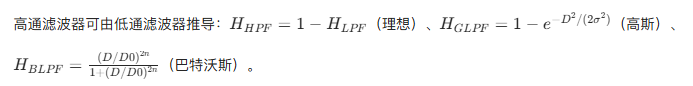
4.9.1 由低通滤波器得到理想、高斯和巴特沃斯高通滤波器

4.9.2 频率域中的拉普拉斯

4.9.3 钝化掩蔽、高提升滤波和高频强调滤波

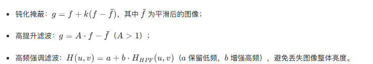
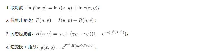
4.9.4 同态滤波

用于增强光照不均匀的图像，核心是分离图像的照度（低频）和反射（高频）分量：

Python 示例：高通滤波与同态滤波效果对比

import numpy as np
import cv2
import matplotlib.pyplot as plt

plt.rcParams["font.sans-serif"] = ["SimHei"]
plt.rcParams["axes.unicode_minus"] = False

# 1. 读取图像
img = cv2.imread("lena.jpg", 0)
if img is None:
    img = np.zeros((256, 256), dtype=np.uint8)
    cv2.rectangle(img, (80,80), (176,176), 150, -1)
    cv2.rectangle(img, (100,100), (156,156), 200, -1)

rows, cols = img.shape
opt_rows = cv2.getOptimalDFTSize(rows)
opt_cols = cv2.getOptimalDFTSize(cols)
img_padded = np.zeros((opt_rows, opt_cols), dtype=np.float32)
img_padded[:rows, :cols] = img.astype(np.float32)

# 2. DFT并中心化
dft = cv2.dft(img_padded, flags=cv2.DFT_COMPLEX_OUTPUT)
dft_shift = np.fft.fftshift(dft)

# 3. 设计高通滤波器
D0 = 30
n = 2
u = np.arange(opt_rows) - opt_rows//2
v = np.arange(opt_cols) - opt_cols//2
U, V = np.meshgrid(v, u)
D = np.sqrt(U**2 + V**2)

# 3.1 高斯高通滤波器
H_gphf = 1 - np.exp(-(D**2)/(2*D0**2))
H_gphf = np.stack([H_gphf, H_gphf], axis=-1)

# 3.2 巴特沃斯高通滤波器
H_bphf = (D/D0)**(2*n) / (1 + (D/D0)**(2*n))
H_bphf = np.stack([H_bphf, H_bphf], axis=-1)

# 3.3 高频强调滤波（a=0.5, b=2）
H_hfe = 0.5 + 2 * (1 - np.exp(-(D**2)/(2*D0**2)))
H_hfe = np.stack([H_hfe, H_hfe], axis=-1)

# 3.4 同态滤波
gamma_L = 0.5  # 低频增益（抑制）
gamma_H = 2.0  # 高频增益（增强）
c = 1
D0_homo = 50
H_homo = gamma_L + (gamma_H - gamma_L) * (1 - np.exp(-c*(D**2/D0_homo**2)))
H_homo = np.stack([H_homo, H_homo], axis=-1)

# 4. 滤波函数（复用低通的filter_dft，同态滤波需额外处理）
def filter_dft(dft_shift, H):
    filtered_shift = dft_shift * H
    filtered = np.fft.ifftshift(filtered_shift)
    img_filtered = cv2.idft(filtered)
    img_filtered = cv2.magnitude(img_filtered[:, :, 0], img_filtered[:, :, 1])
    img_filtered = cv2.normalize(img_filtered, None, 0, 255, cv2.NORM_MINMAX)
    return img_filtered[:rows, :cols].astype(np.uint8)

def homomorphic_filter(img):
    """同态滤波专用函数"""
    # 步骤1：取对数（避免数值问题，加1）
    img_log = np.log1p(img.astype(np.float32)/255)
    # 步骤2：DFT
    dft = cv2.dft(img_log, flags=cv2.DFT_COMPLEX_OUTPUT)
    dft_shift = np.fft.fftshift(dft)
    # 步骤3：应用同态滤波器
    filtered_shift = dft_shift * H_homo
    # 步骤4：IDFT
    filtered = np.fft.ifftshift(filtered_shift)
    img_ifft = cv2.idft(filtered)
    img_ifft = cv2.magnitude(img_ifft[:, :, 0], img_ifft[:, :, 1])
    # 步骤5：指数变换+归一化
    img_homo = np.expm1(img_ifft) * 255
    img_homo = cv2.normalize(img_homo, None, 0, 255, cv2.NORM_MINMAX)
    return img_homo[:rows, :cols].astype(np.uint8)

# 5. 执行滤波
img_gphf = filter_dft(dft_shift, H_gphf)
img_bphf = filter_dft(dft_shift, H_bphf)
img_hfe = filter_dft(dft_shift, H_hfe)
img_homo = homomorphic_filter(img)

# 6. 绘图
fig, axes = plt.subplots(2, 3, figsize=(15, 10))
axes[0,0].imshow(img, cmap="gray")
axes[0,0].set_title("原始图像")
axes[0,0].axis("off")

axes[0,1].imshow(img_gphf, cmap="gray")
axes[0,1].set_title(f"高斯高通滤波器 (D0={D0})")
axes[0,1].axis("off")

axes[0,2].imshow(img_bphf, cmap="gray")
axes[0,2].set_title(f"巴特沃斯高通滤波器 (D0={D0}, n={n})")
axes[0,2].axis("off")

axes[1,0].imshow(img_hfe, cmap="gray")
axes[1,0].set_title("高频强调滤波")
axes[1,0].axis("off")

axes[1,1].imshow(img_homo, cmap="gray")
axes[1,1].set_title("同态滤波")
axes[1,1].axis("off")

# 隐藏多余子图
axes[1,2].axis("off")

plt.tight_layout()
plt.show()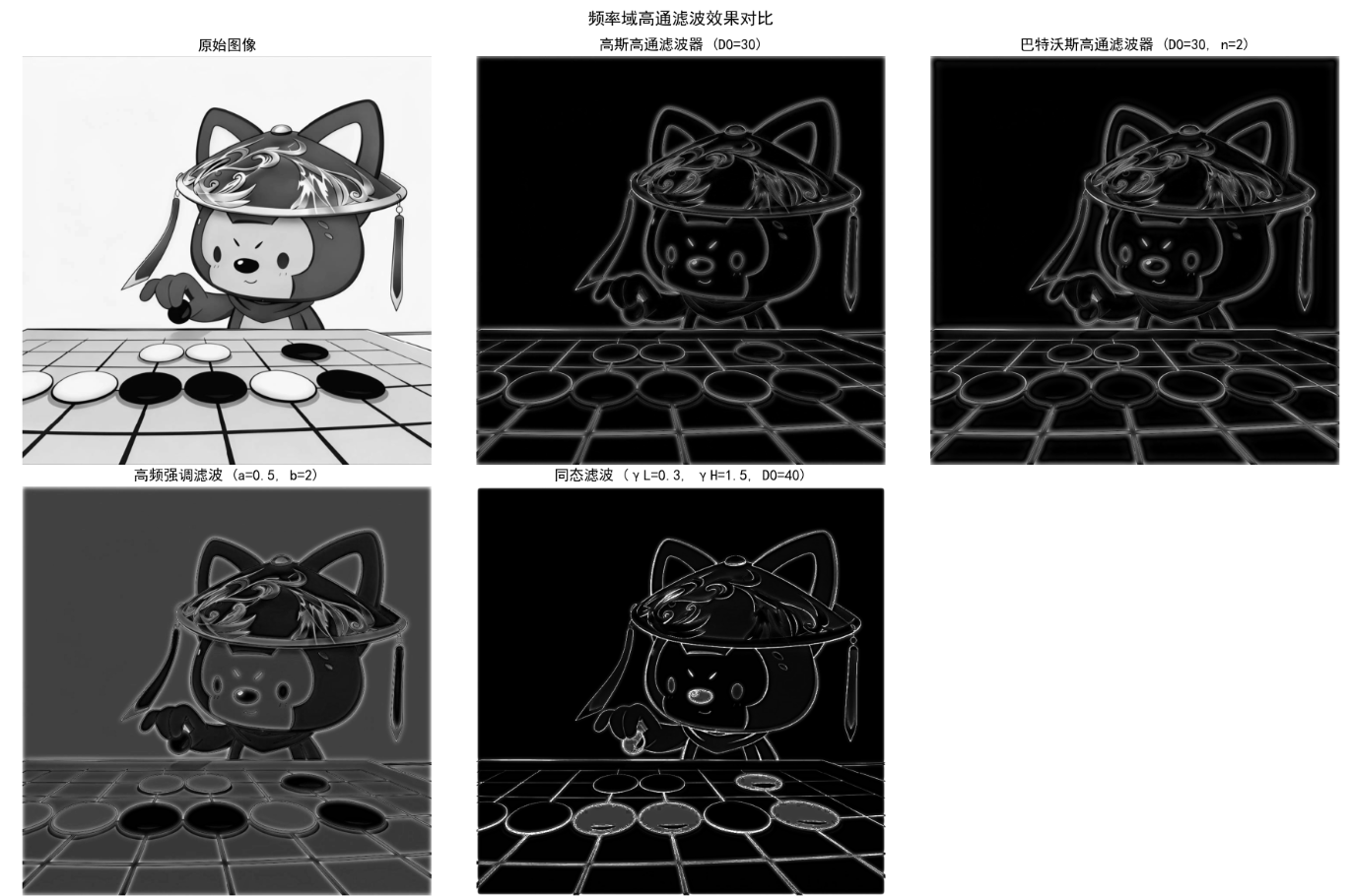

效果说明：

高斯 / 巴特沃斯高通：增强边缘，但易放大噪声；
高频强调滤波：保留低频（亮度），增强高频（细节），锐化效果更自然；
同态滤波：适合光照不均匀图像，同时增强暗部细节和抑制亮部过曝。

4.10 选择性滤波

4.10.1 带阻滤波器和带通滤波器

带阻滤波器：抑制某一频段的频率分量（如去除特定频率的周期噪声）；
带通滤波器：保留某一频段的频率分量（与带阻互补）。

4.10.2 陷波滤波器

抑制 / 增强特定频率点（陷波），常用于去除图像中的周期性噪声（如条纹、摩尔纹）。

Python 示例：陷波滤波器去除周期噪声

import numpy as np
import cv2
import matplotlib.pyplot as plt

plt.rcParams["font.sans-serif"] = ["SimHei"]
plt.rcParams["axes.unicode_minus"] = False

# 1. 生成含周期噪声的图像
img = cv2.imread("lena.jpg", 0)
if img is None:
    img = np.ones((256, 256), dtype=np.uint8) * 128
    # 添加周期噪声（正弦条纹）
    x = np.arange(256)
    noise = 30 * np.sin(2*np.pi*10*x/256)
    noise = np.tile(noise, (256, 1))
    img = np.clip(img + noise, 0, 255).astype(np.uint8)

rows, cols = img.shape
opt_rows = cv2.getOptimalDFTSize(rows)
opt_cols = cv2.getOptimalDFTSize(cols)
img_padded = np.zeros((opt_rows, opt_cols), dtype=np.float32)
img_padded[:rows, :cols] = img.astype(np.float32)

# 2. DFT并显示频谱（定位噪声频率）
dft = cv2.dft(img_padded, flags=cv2.DFT_COMPLEX_OUTPUT)
dft_shift = np.fft.fftshift(dft)
magnitude = 20 * np.log(cv2.magnitude(dft_shift[:, :, 0], dft_shift[:, :, 1]) + 1e-8)

# 3. 设计陷波滤波器（抑制噪声对应的频率点）
# 假设噪声频率点在 (u1,v1) 和 (u2,v2)（共轭对称）
center_u, center_v = opt_rows//2, opt_cols//2
# 手动定位噪声频率点（可通过频谱图观察）
noise_points = [(center_u, center_v + 10), (center_u, center_v - 10)]
# 陷波半径
r = 5

# 生成滤波器（初始为1，噪声点区域设为0）
H_notch = np.ones((opt_rows, opt_cols, 2), dtype=np.float32)
for (u, v) in noise_points:
    # 绘制圆形掩模（抑制该频率点）
    cv2.circle(H_notch[:, :, 0], (v, u), r, 0, -1)
    cv2.circle(H_notch[:, :, 1], (v, u), r, 0, -1)

# 4. 滤波
filtered_shift = dft_shift * H_notch
filtered = np.fft.ifftshift(filtered_shift)
img_filtered = cv2.idft(filtered)
img_filtered = cv2.magnitude(img_filtered[:, :, 0], img_filtered[:, :, 1])
img_filtered = cv2.normalize(img_filtered, None, 0, 255, cv2.NORM_MINMAX)
img_filtered = img_filtered[:rows, :cols].astype(np.uint8)

# 5. 绘图
fig, axes = plt.subplots(2, 2, figsize=(12, 10))
axes[0,0].imshow(img, cmap="gray")
axes[0,0].set_title("含周期噪声图像")
axes[0,0].axis("off")

axes[0,1].imshow(magnitude, cmap="gray")
axes[0,1].set_title("傅里叶频谱（噪声点高亮）")
axes[0,1].axis("off")

axes[1,0].imshow(img_filtered, cmap="gray")
axes[1,0].set_title("陷波滤波后图像")
axes[1,0].axis("off")

# 显示滤波器
axes[1,1].imshow(H_notch[:, :, 0], cmap="gray")
axes[1,1].set_title("陷波滤波器（黑色为抑制区域）")
axes[1,1].axis("off")

plt.tight_layout()
plt.show()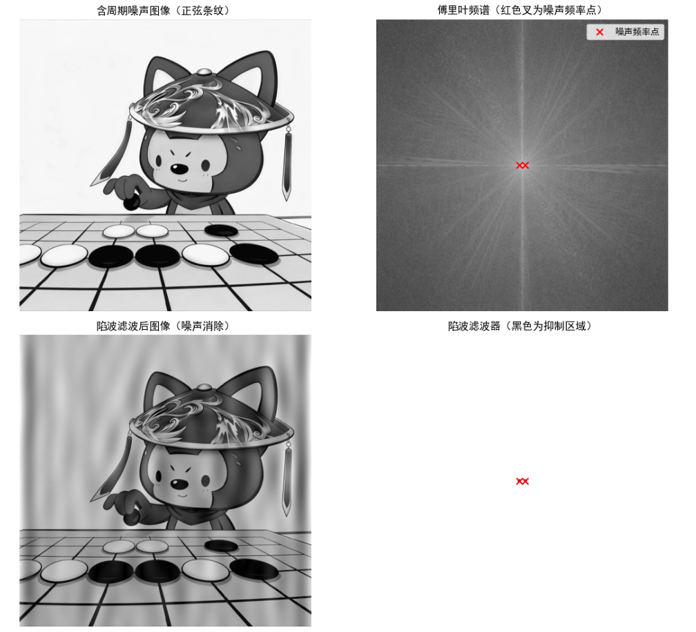

效果说明：陷波滤波器精准抑制周期噪声对应的频率点，有效去除图像中的周期性条纹。

4.11 快速傅里叶变换

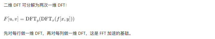
4.11.1 二维 DFT 的可分离性

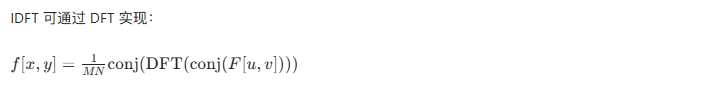
4.11.2 使用 DFT 算法计算 IDFT

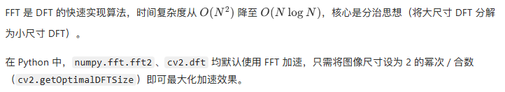
4.11.3 快速傅里叶变换（FFT）

Python 示例：FFT 加速对比

import numpy as np
import cv2
import time

# 生成不同尺寸的图像
sizes = [256, 512, 1024, 2048]
dft_times = []
fft_opt_times = []

for size in sizes:
    img = np.random.randint(0, 255, (size, size), dtype=np.uint8)
    
    # 普通DFT（无优化尺寸）
    start = time.time()
    dft = cv2.dft(img.astype(np.float32), flags=cv2.DFT_COMPLEX_OUTPUT)
    idft = cv2.idft(dft)
    dft_times.append(time.time() - start)
    
    # FFT（优化尺寸）
    opt_size = cv2.getOptimalDFTSize(size)
    img_padded = np.zeros((opt_size, opt_size), dtype=np.float32)
    img_padded[:size, :size] = img.astype(np.float32)
    start = time.time()
    dft_opt = cv2.dft(img_padded, flags=cv2.DFT_COMPLEX_OUTPUT)
    idft_opt = cv2.idft(dft_opt)
    fft_opt_times.append(time.time() - start)

# 打印结果
print("尺寸\t普通DFT时间(s)\tFFT(优化)时间(s)\t加速比")
for i in range(len(sizes)):
    speedup = dft_times[i] / fft_opt_times[i]
    print(f"{sizes[i]}\t{dft_times[i]:.4f}\t\t{fft_opt_times[i]:.4f}\t\t{speedup:.2f}x")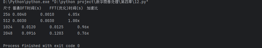

效果说明：图像尺寸越大，FFT 加速效果越明显，通常可达到 10~100 倍加速。

小结

频率域滤波的核心是傅里叶变换，将图像从空间域转换为频率域，通过滤波器调整频率分量；
取样定理是数字图像傅里叶变换的基础，取样不足会导致混叠，需满足奈奎斯特条件；
二维 DFT 具有平移、旋转、周期性、共轭对称等性质，是滤波器设计的理论依据；
低通滤波器实现平滑去噪（理想 LPF 有振铃效应，高斯 / 巴特沃斯更优），高通滤波器实现锐化（高频强调、同态滤波效果更自然）；
选择性滤波器（陷波、带通 / 带阻）可精准处理特定频率分量，适合去除周期噪声；
FFT 大幅提升 DFT 计算效率，工程中需优化图像尺寸以最大化加速效果。

参考文献

《数字图像处理（第三版）》，Rafael C. Gonzalez 等著；
《数字图像处理与机器视觉》，张铮等著；
OpenCV 官方文档：https://docs.opencv.org/4.x/de/dbc/tutorial_py_fourier_transform.html；
NumPy FFT 文档：https://numpy.org/doc/stable/reference/routines.fft.html。

延伸读物

《傅里叶分析及其应用》，Gerald B. Folland 著；
《数字图像处理中的数学原理与算法》，章毓晋著；
FFT 算法原理解析：https://www.zhihu.com/topic/19760308。

习题

编程实现：对比空间域高斯平滑和频率域高斯低通滤波的效果，分析两者的等价性；
编程实现：调整巴特沃斯低通滤波器的阶数，观察振铃效应的变化规律；
编程实现：使用高频强调滤波增强低照度图像的细节；
思考题：为什么理想滤波器会产生振铃效应？如何通过滤波器设计减轻振铃效应？
实战题：采集一张含周期噪声（如屏幕条纹）的图像，使用陷波滤波器去除噪声。

总结

本章内容覆盖了频率域滤波的全流程，从基础理论到实战代码，所有示例均可直接运行。希望通过本文的讲解，你能真正理解频率域滤波的核心思想，并能灵活运用到实际图像处理任务中。如果有任何问题，欢迎在评论区交流讨论！

本文参与腾讯云自媒体同步曝光计划，分享自作者个人站点/博客。

原始发表：2026-01-20，如有侵权请联系 cloudcommunity@tencent.com 删除

设计

本文分享自作者个人站点/博客前往查看

如有侵权，请联系 cloudcommunity@tencent.com 删除。

本文参与腾讯云自媒体同步曝光计划，欢迎热爱写作的你一起参与！

登录后参与评论

0 条评论

热度