单细胞韧皮部研究代码解析2--comparison_denyer2019.R
原创
单细胞韧皮部研究代码解析2--comparison_denyer2019.R
原创
小胡子刺猬的生信学习123
发布于 2023-04-08 18:16:23
发布于 2023-04-08 18:16:23
单细胞韧皮部研究代码解析1-QC_filtering.R:https://cloud.tencent.com/developer/article/2256814?areaSource=&traceId=
今天继续给大家分享这篇作者的代码,在很多人做单细胞数据分析的时候,,目前是伴随单细胞组学的发展,如何将前人发表的单细胞转录组数据与获得的单细胞数据进行整合,这篇文章的作者提供了一个思路。
代码解析
###data及R包的读入
###作者这里选用的是scater进行后续的分析,这里需要自己提前安装,可以用conda先构建一个scater的环境,后续lib.loc进行调用
library(data.table)
library(scater)
library(scran)
library(ggplot2)
library(patchwork)

# set seed for reproducible results
set.seed(1001)

# set ggplot2 theme
theme_set(theme_bw() + theme(text = element_text(size = 14)))

# source util functions
#这里还是作者在github上分享的自己的R代码,其中有getReducedDim函数,需要提前下载下来
source("analysis/functions/utils.R")

# Marker genes whose promoters were used for cell sorting
markers <- data.table(name = c("APL", "MAKR5", "PEARdel", "S17", "sAPL"),
                      id = c("AT1G79430", "AT5G52870", "AT2G37590", "AT2G22850", "AT3G12730"))


# Read data ---------------------------------------------------------------

# ring data both soft and hard filtered
ring_soft <- readRDS("data/processed/SingleCellExperiment/ring_batches_softfilt.rds")
ring_hard <- readRDS("data/processed/SingleCellExperiment/ring_batches_hardfilt.rds")

# all batches, both soft and hard filtered
all_soft <- readRDS("data/processed/SingleCellExperiment/all_batches_softfilt.rds")
all_soft$dataset <- ifelse(grepl("denyer", all_soft$Sample), "Denyer et al 2019", "ring")

all_hard <- readRDS("data/processed/SingleCellExperiment/all_batches_hardfilt.rds")
all_hard$dataset <- ifelse(grepl("denyer", all_hard$Sample), "Denyer et al 2019", "ring")


# Comparison with Denyer - hard filter ------------------------------------

# plot things together
##作者前面已经确定了UMAP-MNN_30是最符合自己数据集的降维方式,所以这里自己调用的时候需要更改
##这里是根据ggthemes这个包的不同颜色进行填充对上面读入的all_hard data 进行可视化:scale_colour_tableau
p1 <- ggplot(getReducedDim(all_hard, "UMAP-MNN_30"), aes(V1, V2, group = cluster_mnn)) +
  geom_point(aes(colour = cluster_mnn), show.legend = FALSE) +
  geom_label(stat = "centroid", aes(label = cluster_mnn), size = 3,
             label.padding = unit(0.1, "lines")) +
  ggthemes::scale_colour_tableau(palette = "Tableau 20") +
  labs(x = "UMAP 1", y = "UMAP 2")

p2 <- ggplot(getReducedDim(all_hard, "UMAP-MNN_30"), aes(V1, V2)) +
  geom_point(aes(colour = dataset)) +
  labs(x = "UMAP 1", y = "UMAP 2") +
  scale_colour_brewer(palette = "Dark2")

p3 <- ggplot(getReducedDim(all_hard, "UMAP-MNN_30"), aes(V1, V2)) +
  ggpointdensity::geom_pointdensity(show.legend = FALSE) +
  labs(x = "UMAP 1", y = "UMAP 2") +
  scale_colour_viridis_c(option = "magma") +
  facet_grid(~ dataset)

(p1 | p2) / p3 + plot_annotation(tag_levels = "A") + plot_layout(guides = "collect")


# plot genes mentioned in Denyer2019 Fig 2D
temp <- getReducedDim(all_hard, "UMAP-MNN_30", genes = c("AT3G58190", "AT1G79430", "AT5G47450"),
              melted = TRUE)
ggplot(temp[order(expr, na.last = FALSE)], aes(V1, V2)) +
  geom_point(aes(colour = expr)) +
  scale_colour_viridis_c() +
  facet_grid(dataset ~ id) +
  labs(x = "UMAP 1", y = "UMAP 2")


# Comparison with Denyer - soft filter -------------------------------------
***
# plot things together
# cluster_mnn:这里是作者的分群数据
# dataset:拟整合的Denyer 的数据集
p1 <- ggplot(getReducedDim(all_soft, "UMAP-MNN_30"), aes(V1, V2, group = cluster_mnn)) +
  geom_point(aes(colour = cluster_mnn), show.legend = FALSE) +
  geom_label(stat = "centroid", aes(label = cluster_mnn), size = 3,
             label.padding = unit(0.1, "lines")) +
  ggthemes::scale_colour_tableau(palette = "Tableau 20") +
  labs(x = "UMAP 1", y = "UMAP 2")

p2 <- ggplot(getReducedDim(all_soft, "UMAP-MNN_30"), aes(V1, V2)) +
  geom_point(aes(colour = dataset)) +
  labs(x = "UMAP 1", y = "UMAP 2") +
  scale_colour_brewer(palette = "Dark2")

p3 <- ggplot(getReducedDim(all_soft, "UMAP-MNN_30"), aes(V1, V2)) +
  ggpointdensity::geom_pointdensity(show.legend = FALSE) +
  labs(x = "UMAP 1", y = "UMAP 2") +
  scale_colour_viridis_c(option = "magma") +
  facet_grid(~ dataset)

(p1 | p2) / p3 + plot_annotation(tag_levels = "A") + plot_layout(guides = "collect")
***

# plot genes mentioned in Denyer2019 Fig 2D
# 选取部分已知的marker 基因进行可视化
temp <- getReducedDim(all_soft, "UMAP-MNN_30", genes = c("AT3G58190", "AT1G79430", "AT5G47450"),
                      melted = TRUE)
temp$expr <- ifelse(temp$expr == 0, NA, temp$expr)
ggplot(temp[order(expr, na.last = FALSE)], aes(V1, V2)) +
  geom_point(aes(colour = expr)) +
  scale_colour_viridis_c() +
  facet_grid(dataset ~ id) +
  labs(x = "UMAP 1", y = "UMAP 2")


# Contaminating layers ----------------------------------------------------
# plot genes identifying collumela and epidermis
# 选用已知的中柱和表皮的marker 基因,对all_hard和all_soft数据集进行可视化

# hard filtered data
temp <- getReducedDim(all_hard, "UMAP-MNN_30",
                      genes = c("AT1G79580", "AT3G29810", "AT5G58580", "AT5G14750"),
                      melted = TRUE)
temp$expr <- ifelse(temp$expr == 0, NA, temp$expr)
ggplot(temp[order(expr, na.last = FALSE)], aes(V1, V2)) +
  geom_point(aes(colour = expr)) +
  scale_colour_viridis_c() +
  facet_grid(dataset ~ id) +
  labs(x = "UMAP 1", y = "UMAP 2")


# soft filtered data
temp <- getReducedDim(all_soft, "UMAP-MNN_30",
                      genes = c("AT1G79580", "AT3G29810", "AT5G58580", "AT5G14750"),
                      melted = TRUE)
temp$expr <- ifelse(temp$expr == 0, NA, temp$expr)
ggplot(temp[order(expr, na.last = FALSE)], aes(V1, V2)) +
  geom_point(aes(colour = expr)) +
  scale_colour_viridis_c() +
  facet_grid(dataset ~ id) +
  labs(x = "UMAP 1", y = "UMAP 2")


# Collumela
temp <- getReducedDim(all_hard, "UMAP-MNN_30", genes = c("AT1G79580", "AT1G13620", "AT2G04025"),
                      melted = TRUE)
ggplot(temp[order(expr, na.last = FALSE)], aes(V1, V2)) +
  geom_point(aes(colour = expr)) +
  scale_colour_viridis_c() +
  facet_grid(dataset ~ id) +
  labs(x = "UMAP 1", y = "UMAP 2")

# Epidermis - actually AT2G46410 is also expressed in "stele"
# https://www.ncbi.nlm.nih.gov/pmc/articles/PMC150583/
temp <- getReducedDim(all_hard, "UMAP-MNN_30", genes = c("AT5G14750", "AT1G79840", "AT2G46410"),
                      melted = TRUE)
ggplot(temp[order(expr, na.last = FALSE)], aes(V1, V2)) +
  geom_point(aes(colour = expr)) +
  scale_colour_viridis_c() +
  facet_grid(dataset ~ id) +
  labs(x = "UMAP 1", y = "UMAP 2")

# Genes used for sorting
# 前期用于分选的marker基因进行可视化
temp <- getReducedDim(all_hard, "UMAP-MNN_30",
                      genes = unique(markers$id), melted = TRUE)
temp <- merge(temp, markers, by = "id")
ggplot(temp[order(expr, na.last = FALSE)], aes(V1, V2)) +
  geom_point(aes(colour = expr)) +
  scale_colour_viridis_c() +
  facet_grid(dataset ~ name) +
  labs(x = "UMAP 1", y = "UMAP 2")
总结
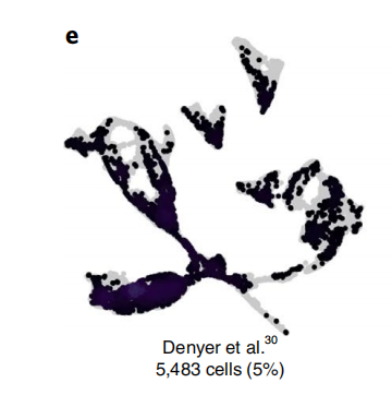
通过前面的代码解析,发现是作者是提前把denyer的数据进行了整合,主要的可视化的代码是*** ***里面的内容。首先时作者读入了soft和hard 的data,把自己以前进行分选的marker基因及已知的marker基因进行整合数据集的可视化,去表明整合后的数据集都能定位到相似的位置,验证自己的数据集的可靠性。
原创声明:本文系作者授权腾讯云开发者社区发表,未经许可,不得转载。
如有侵权,请联系 cloudcommunity@tencent.com 删除。
原创声明:本文系作者授权腾讯云开发者社区发表,未经许可,不得转载。
如有侵权,请联系 cloudcommunity@tencent.com 删除。
评论
登录后参与评论
推荐阅读
目录
腾讯云开发者

Copyright © 2013 - 2026 Tencent Cloud. All Rights Reserved. 腾讯云 版权所有
深圳市腾讯计算机系统有限公司 ICP备案/许可证号:粤B2-20090059 ![]() 粤公网安备44030502008569号
粤公网安备44030502008569号
腾讯云计算(北京)有限责任公司 京ICP证150476号 | 京ICP备11018762号