xarray基础之计算篇


import xarray as xr
# 数据
f = '/home/mw/input/cru3546/cru_ts4.07.2021.2022.pre.dat.nc'

# 打开数据集
ds = xr.open_dataset(f)
dsWarning: ecCodes 2.21.0 or higher is recommended. You are running version 2.14.1平均
In [12]:
all_mean_pre = ds.pre.mean()

print('两年全球平均降水:', all_mean_pre)两年全球平均降水: <xarray.DataArray 'pre' ()>
array(61.810722, dtype=float32)In [10]:
first_mean_pre = ds.pre.sel(time=slice('2021-01-16', '2021-12-16')).mean()

print('2021年全球平均降水:', first_mean_pre)2021年全球平均降水: <xarray.DataArray 'pre' ()>
array(61.74274, dtype=float32)In [17]:
point_mean_pre = ds.pre.sel(time=slice('2021-01-16', '2021-12-16'),lat=32.75,lon=60.25).mean()

print('2021年某格点平均降水:', point_mean_pre)2021年某格点平均降水: <xarray.DataArray 'pre' ()>
array(12.158334, dtype=float32)
Coordinates:
lon float32 60.25
lat float32 32.75总和
In [18]:
sum_pre = ds.pre.sum()
print('两年全球总降水:', sum_pre)两年全球总降水: <xarray.DataArray 'pre' ()>
array(1.00014696e+08, dtype=float32)标准差
In [19]:
std_pre = ds.pre.std()
print('pre std:', std_pre)pre std: <xarray.DataArray 'pre' ()>
array(85.1408844)最大值与最大值坐标
In [24]:
max=ds.pre.max()
maxOut[24]:

In [37]:
argmax=ds.pre.argmax(dim=['lon','lat'])
argmaxOut[37]:
{'lon': <xarray.DataArray 'pre' (time: 24)>
 array([612, 641, 641, 256, 204, 548, 509, 545, 205, 576, 520, 612, 716,
        612, 612, 612, 556, 543, 506, 556, 641, 603, 205, 565])
 Coordinates:
   * time     (time) datetime64[ns] 2021-01-16 2021-02-15 ... 2022-12-16,
 'lat': <xarray.DataArray 'pre' (time: 24)>
 array([199, 170, 170, 189, 185, 216, 207, 220, 188, 212, 205, 199, 144,
        199, 199, 199, 204, 230, 218, 208, 168, 209, 188, 191])
 Coordinates:
   * time     (time) datetime64[ns] 2021-01-16 2021-02-15 ... 2022-12-16}
输出了二十四时间点的最大值坐标,下面选一个时间点
In [51]:
ds.pre[0].max()Out[51]:

In [41]:
ds.pre[0].argmax(dim=['lat','lon'])Out[41]:
{'lat': <xarray.DataArray 'pre' ()>
 array(199)
 Coordinates:
     time     datetime64[ns] 2021-01-16,
 'lon': <xarray.DataArray 'pre' ()>
 array(612)
 Coordinates:
     time     datetime64[ns] 2021-01-16}
In [42]:
ds.pre[0][199,612]Out[42]

上面已找到最大值的经纬度,顺便画个图
In [48]:
import matplotlib.pyplot as plt
import numpy as np
import cartopy.crs as ccrs
import cartopy.feature as cfeature
from cartopy.mpl.ticker import LongitudeFormatter, LatitudeFormatter
from matplotlib.colors import LinearSegmentedColormap
import cmaps
lons=ds.lon
lats=ds.lat
data=ds.pre[0]
fig = plt.figure(figsize=(20,18))

# 设置地图投影为PlateCarree
ax = plt.axes(projection=ccrs.PlateCarree())

# 绘制填充等值线图
cs = ax.contourf(lons, lats, data, transform=ccrs.PlateCarree(), cmap=cmaps.radar, levels=np.linspace(data.min(), data.max(), 20))
# 添加网格线
ax.gridlines(draw_labels=True, dms=True, x_inline=False, y_inline=False)
# 添加海岸线
ax.coastlines()/opt/conda/lib/python3.7/site-packages/cmaps/cmaps.py:3517: UserWarning: Trying to register the cmap 'radar' which already exists.
matplotlib.cm.register_cmap(name=cname, cmap=cmap)Out[48]:
<cartopy.mpl.feature_artist.FeatureArtist at 0x7fa2feef28d0>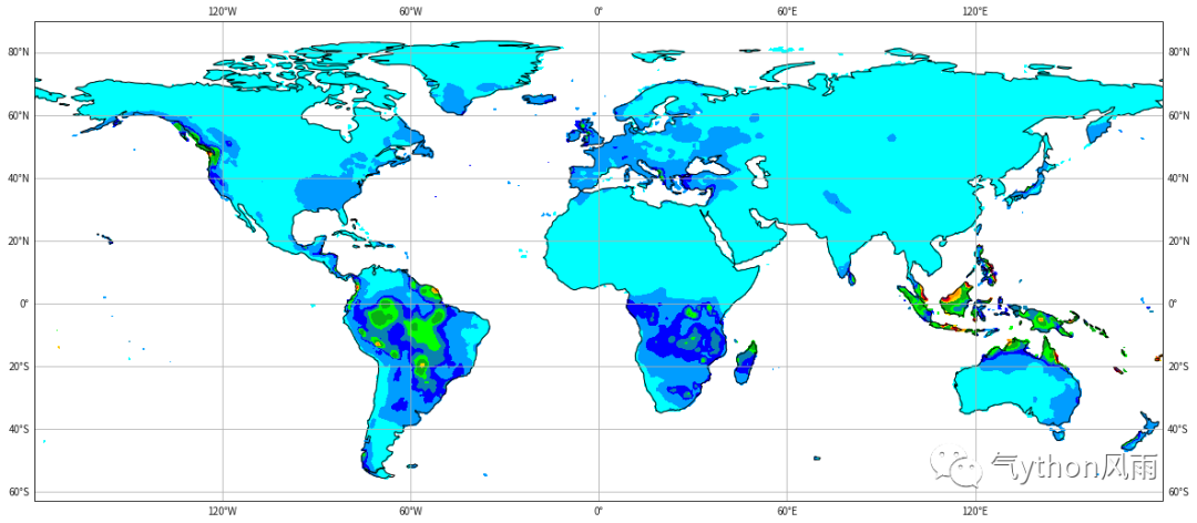
In [57]:
import matplotlib.pyplot as plt
import numpy as np
import cartopy.crs as ccrs
import cartopy.feature as cfeature
from cartopy.mpl.ticker import LongitudeFormatter, LatitudeFormatter
from matplotlib.colors import LinearSegmentedColormap
import cmaps
lons=ds.lon
lats=ds.lat
data=ds.pre[0]
fig = plt.figure(figsize=(20,10))

# 设置地图投影为PlateCarree
ax = plt.axes(projection=ccrs.PlateCarree())

# 绘制填充等值线图
cs = ax.contourf(lons, lats, data, transform=ccrs.PlateCarree(), cmap=cmaps.radar_1, levels=np.linspace(data.min(), data.max(), 20))
# 添加网格线
ax.gridlines(draw_labels=True, dms=True, x_inline=False, y_inline=False)
# 设置经纬度范围
ax.set_extent([120, 130, 5, 15], crs=ccrs.PlateCarree())
# 最大值打点
ax.scatter([data.lon[612]],[data.lat[199]],color='b',s=10)
# 添加海岸线
ax.coastlines()
ax.scatter([data.lon[612]],[data.lat[199]],color='b',s=20)
cbar = plt.colorbar(cs, orientation='vertical')

/opt/conda/lib/python3.7/site-packages/cmaps/cmaps.py:3533: UserWarning: Trying to register the cmap 'radar_1' which already exists.
  matplotlib.cm.register_cmap(name=cname, cmap=cmap)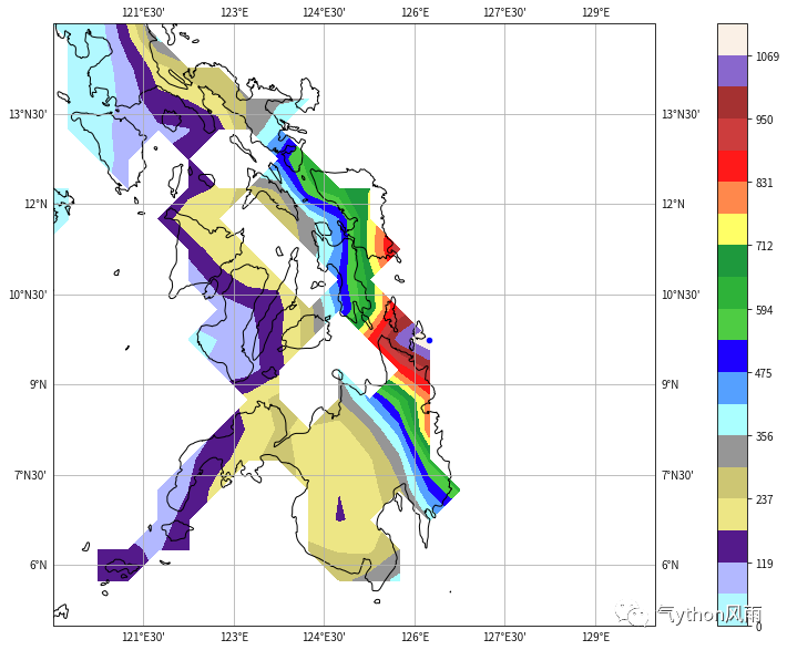
在东经126,北纬9的附近的小黑点就是最大值所在,格点数据放大看确实有点奇形怪状 还有对应的argmin,用法差不多就不多介绍了
获得下月减上月的数组
In [61]:
diff = ds.pre.diff(dim='time')
diff
Out[61]:

diff[0].plot()Out[62]:
<matplotlib.collections.QuadMesh at 0x7fa2fe46a3d0>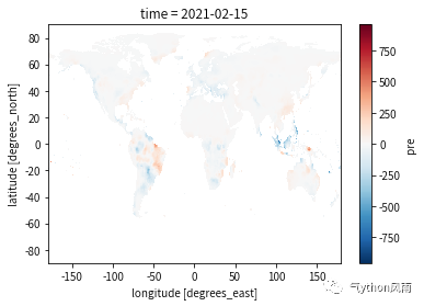
转为pandas计算
In [66]:
df = ds.to_dataframe()
df
Out[66]:
pre | stn | |||
|---|---|---|---|---|
lon | lat | time | ||
-179.75 | -89.75 | 2021-01-16 | NaN | NaN |
2021-02-15 | NaN | NaN | ||
2021-03-16 | NaN | NaN | ||
2021-04-16 | NaN | NaN | ||
2021-05-16 | NaN | NaN | ||
... | ... | ... | ... | ... |
179.75 | 89.75 | 2022-08-16 | NaN | NaN |
2022-09-16 | NaN | NaN | ||
2022-10-16 | NaN | NaN | ||
2022-11-16 | NaN | NaN | ||
2022-12-16 | NaN | NaN |
6220800 rows × 2 columns
均值
In [80]:
mean = df.mean()
mean
Out[80]:
pre    61.771572
stn     4.029309
dtype: float64
指定列最大值
In [81]:
max_value = df['pre'].max()
max_value
Out[81]:
2311.800048828125列总和
In [84]:
sum_by_row = df.sum(axis=0)
sum_by_row
Out[84]:
pre    100014712.0
stn      6519744.0
dtype: float64
标准差与相关系数
In [85]:
std_dev = df.std()
std_dev
Out[85]:
pre    85.079056
stn     3.012599
dtype: float64
In [86]:
correlation = df.corr()
correlation
Out[86]:
pre | stn | |
|---|---|---|
pre | 1.000000 | 0.038891 |
stn | 0.038891 | 1.000000 |
最大值坐标
In [3]:
import pandas as pd
# 转格式
df = ds.to_dataframe()
print(df)
# 查找最大值
max_value = df["pre"].max()
print(max_value)
# 查找最大值所在的时间
idx = df["pre"].idxmax()
idx pre stn
lon lat time
-179.75 -89.75 2021-01-16 NaN NaN
2021-02-15 NaN NaN
2021-03-16 NaN NaN
2021-04-16 NaN NaN
2021-05-16 NaN NaN
... ... ...
179.75 89.75 2022-08-16 NaN NaN
2022-09-16 NaN NaN
2022-10-16 NaN NaN
2022-11-16 NaN NaN
2022-12-16 NaN NaN
[6220800 rows x 2 columns]
2311.800048828125Out[3]:
(74.75, 13.75, Timestamp('2021-07-16 00:00:00'))
本文参与 腾讯云自媒体同步曝光计划,分享自微信公众号。
原始发表:2023-12-31,如有侵权请联系 cloudcommunity@tencent.com 删除
评论
登录后参与评论
推荐阅读
目录
腾讯云开发者

Copyright © 2013 - 2026 Tencent Cloud. All Rights Reserved. 腾讯云 版权所有
深圳市腾讯计算机系统有限公司 ICP备案/许可证号:粤B2-20090059 ![]() 粤公网安备44030502008569号
粤公网安备44030502008569号
腾讯云计算(北京)有限责任公司 京ICP证150476号 | 京ICP备11018762号