课前准备--CODEX(IMC)基础分析梳理
原创
课前准备--CODEX(IMC)基础分析梳理
原创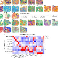
追风少年i
发布于 2025-07-31 09:19:15
发布于 2025-07-31 09:19:15
作者,Evil Genius
我们也来到了空间蛋白组的课程范围了。
为什么做了空间转录组,还要做空间蛋白组,也就是说转录组和蛋白组的对应关系如何,这个多次在课程上谈到了。
CODEX 与 IMC 技术简介
1. CODEX(Co-Detection by indEXing)
原理:基于荧光标记抗体的循环成像技术,通过多轮抗体染色、成像和荧光淬灭,实现高维蛋白检测(可检测40-100+蛋白)。
特点:
- 使用 荧光标记抗体,兼容常规显微镜(无需特殊设备)。
- 高分辨率(亚细胞级),适合 组织微环境的空间分析。
- 适用于 新鲜冷冻或FFPE(福尔马林固定石蜡包埋)样本。
2. IMC(Imaging Mass Cytometry)
原理:基于 质谱流式(CyTOF) 技术,使用金属同位素标记抗体,通过激光剥蚀+质谱检测实现高维蛋白成像(通常检测30-50种蛋白)。
特点:
- 无荧光干扰,信号重叠极低,适合超高复用检测。
- 分辨率略低于CODEX(~1µm vs. CODEX的亚微米级)。
- 仅适用于 FFPE样本(需特殊制备)。
CODEX 与 IMC 的主要差异
对比维度 | CODEX | IMC |
|---|---|---|
检测原理 | 荧光标记抗体 + 多轮成像 | 金属同位素标记抗体 + 质谱检测 |
检测通量 | 40-100+ 种蛋白 | 30-50 种蛋白(受限于金属同位素) |
分辨率 | 亚微米级(~0.3µm) | ~1µm(略低于CODEX) |
样本兼容性 | 新鲜冷冻、FFPE | 仅FFPE |
信号干扰 | 可能存在荧光串扰 | 无串扰(质谱检测) |
设备需求 | 荧光显微镜 + 自动化成像系统 | 激光剥蚀 + 质谱流式(CyTOF)设备 |
数据分析 | 基于荧光信号的多维解卷积 | 基于质谱峰值的空间成像 |
适用场景 | 高分辨率、多轮检测的微环境研究 | 超高复用、无背景干扰的蛋白检测 |
CODEX 更适合 高分辨率、多轮检测 的空间蛋白组研究,尤其适用于 细胞互作和微环境分析。
IMC 更适合 超高复用、无背景干扰 的蛋白检测,但分辨率略低,且依赖 FFPE样本。
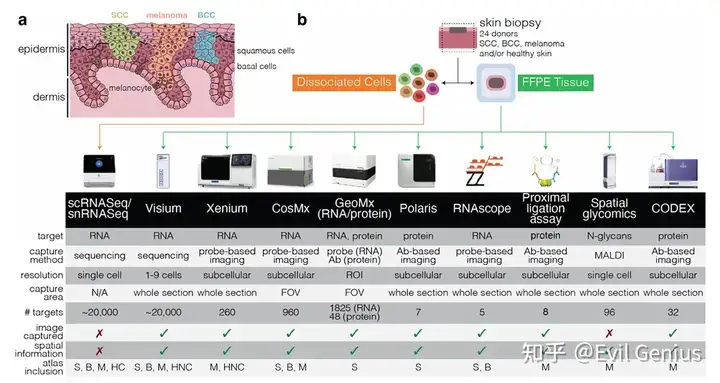
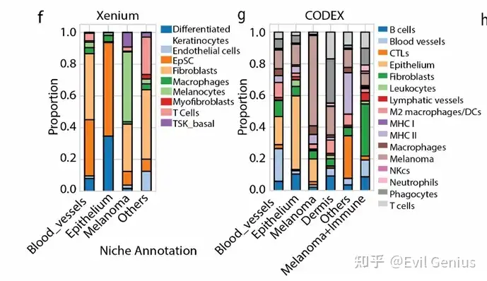
多技术比较
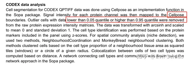
关于CODEX常见的数据质控,与普通的转录组有些区别
当然了,对于空间组学而言,niche分析是必不可少的。
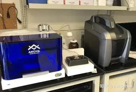
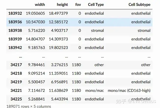
大家分析的时候,一般交付了的数据是cell_by_gene.csv和cellmetadata.csv,空间那种抗体图需要机器上展示。
基础分析参考网址Monkeybread Tutorial — Monkeybread
我们来总结一下分析代码
import sys
import subprocess
import numpy as np
import pandas as pd
import scanpy as sc
import anndata
from anndata import AnnData
from matplotlib import pyplot as plt
import matplotlib as mpl
import seaborn as sns
import os

import monkeybread as mb
读取的数据仍然是h5ad格式
sc.pp.normalize_total(adata, inplace=True)
sc.pp.log1p(adata)
sc.pp.pca(adata)
# Display high-level cell types
fig, ax = plt.subplots(1, 1, figsize=(5,5))
sc.pl.embedding(
adata,
"spatial",
color = 'Cell Type',
s=1,
ax=ax,
palette=sc.pl.palettes.vega_20_scanpy,
show=False
)
plt.show()
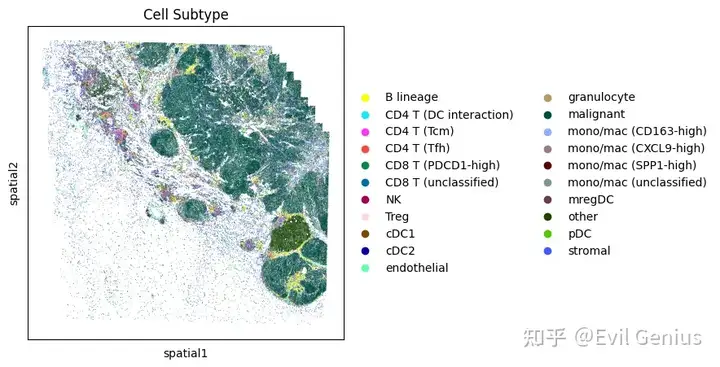
# Display more granular cell subtypes
fig, ax = plt.subplots(1, 1, figsize=(5,5))
sc.pl.embedding(
adata,
"spatial",
color = 'Cell Subtype',
s=1,
ax=ax,
palette=sc.pl.palettes.godsnot_102,
show=False
)
plt.show()
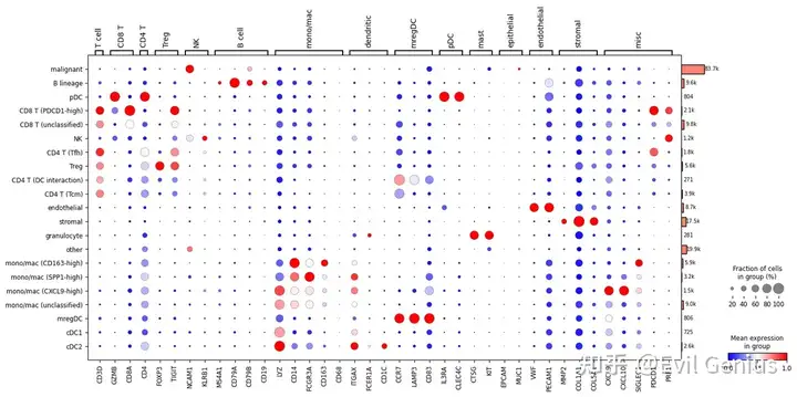
# Display expression dotplot
sc.tl.dendrogram(adata, groupby='Cell Subtype')
dp = sc.pl.dotplot(
adata,
var_names={
'T cell': [
'CD3D'
],
'CD8 T': [
'GZMB',
'CD8A'
],
'CD4 T': [
'CD4'
],
'Treg': [
'FOXP3',
'TIGIT'
],
'NK': [
'NCAM1',
'KLRB1'
],
'B cell': [
'MS4A1',
'CD79A',
'CD79B',
'CD19'
],
'mono/mac': [
'LYZ',
'CD14',
'FCGR3A',
'CD163',
'CD68'
],
'dendritic': [
'ITGAX',
'FCER1A',
'CD1C'
],
'mregDC': [
'CCR7',
'LAMP3',
'CD83'
],
'pDC': [
'IL3RA',
'CLEC4C'
],
'mast': [
'CTSG',
'KIT'
],
'epithelial': [
'EPCAM',
'MUC1'
],
'endothelial': [
'VWF',
'PECAM1'
],
'stromal': [
'MMP2',
'COL1A1',
'COL5A1'
],
'misc': [
'CXCL9',
'CXCL10',
'SIGLEC1',
'PDCD1',
'PRF1'
]
},
groupby=['Cell Subtype'],
standard_scale='var',
cmap='bwr',
dendrogram=True,
return_fig=True
)
dp.add_totals().show()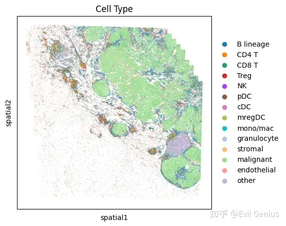
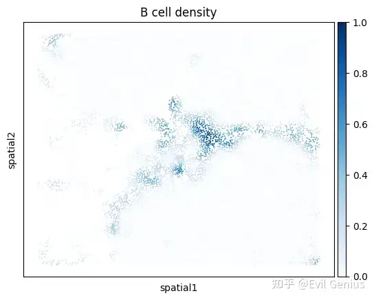
Plot density of cells of a given cell type
density_key = mb.calc.cell_density(
    adata_zoom,
    'Cell Type',
    'B lineage',
    bandwidth=25,
    approx=False,
    radius_threshold=250
)
mb.plot.cell_density(
    adata_zoom,
    density_key,
    cmap='Blues',
    title=f'B cell density'
)
fig, _ = mb.plot.location_and_density(
    adata,
    'Cell Subtype',
    [
        ['B lineage'],  # The first group of cell types to plot
        ['CD4 T (Tfh)'] # The second group of cell types to plot
    ],
    [
        'B cell', # Name of the first group of cell types
        'CD4 Tfh' # Name of the second group of cell types
    ],
    dot_size=[1, 1], # Dot sizes for each group
    title='B cell vs. CD4 Tfh',
    grid=True,
    n_grids=5,
    show=False
)
plt.tight_layout()
plt.show()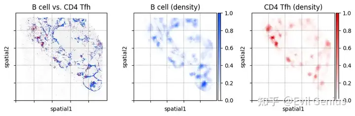
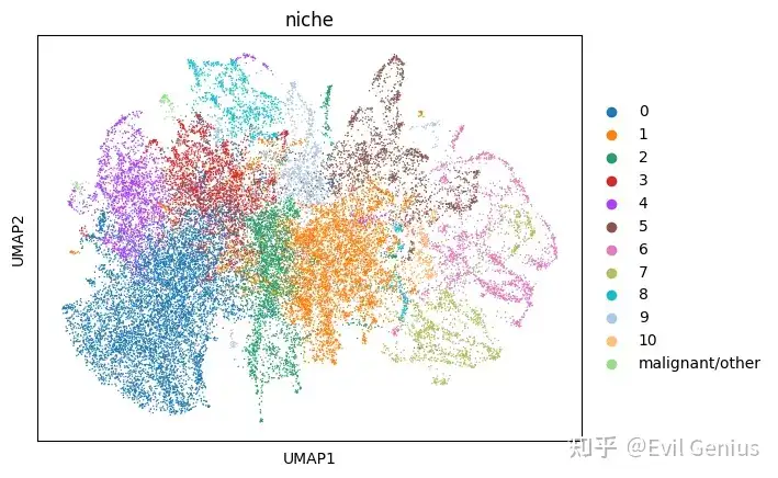
Niche analysis
niche_subtypes = []
other_cell_types = ['other', 'malignant']
for cell, ct in zip(adata.obs.index, adata.obs['Cell Subtype']):
    if ct in other_cell_types:
        niche_subtypes.append('malignant/other')
    else:
        niche_subtypes.append(ct)
adata.obs['niche_subtypes'] = niche_subtypes
adata.obs['niche_subtypes'] = adata.obs['niche_subtypes'].astype('category')

print("Cell subtypes considered in niche analysis:")
print(set(adata.obs['niche_subtypes']))
# Only perform niche analysis on immune cells
immune_mask = ~adata.obs['niche_subtypes'].isin([
    'malignant/other', 'endothelial', 'stromal'
])

# Compute niches
adata_neighbors = mb.calc.cellular_niches(
    adata,
    cell_type_key='niche_subtypes',
    radius=75,
    normalize_counts=True,
    standard_scale=True,
    clip_min=-5,
    clip_max=5,
    mask=immune_mask,
    n_neighbors=100,
    resolution=0.25,
    min_niche_size=300,
    key_added='niche',
    non_niche_value='malignant/other'
)

# Subset cells
adata_neighbors_sub = sc.pp.subsample(
    adata_neighbors, fraction=1/2, copy=True
)

# Generate UMAP plots
sc.tl.umap(adata_neighbors_sub)
sc.pl.umap(
    adata_neighbors_sub,
    color='niche_subtypes',
    palette=sc.pl.palettes.vega_20_scanpy
)
sc.pl.umap(
    adata_neighbors_sub,
    color='niche',
    palette=sc.pl.palettes.vega_20_scanpy
)
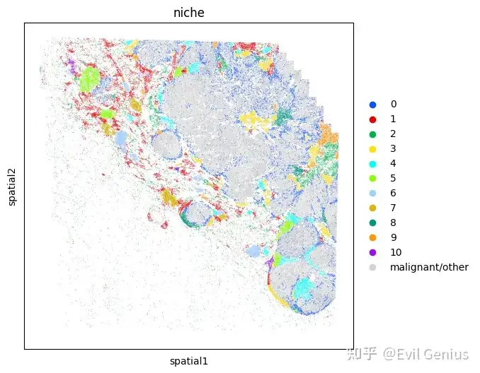
# Map each niche to a color so that plots are consistent
niche_to_color = {
    val: mb.plot.monkey_palette[i]
    for i, val in enumerate(sorted(set(adata_neighbors.obs['niche'])))
}
niche_to_color['malignant/other'] = 'lightgrey'

fig, ax = plt.subplots(1,1,figsize=(6,6))
sc.pl.embedding(
    adata,
    "spatial",
    color = 'niche',
    palette=niche_to_color,
    s=1,
    ax=ax,
    show=False
)
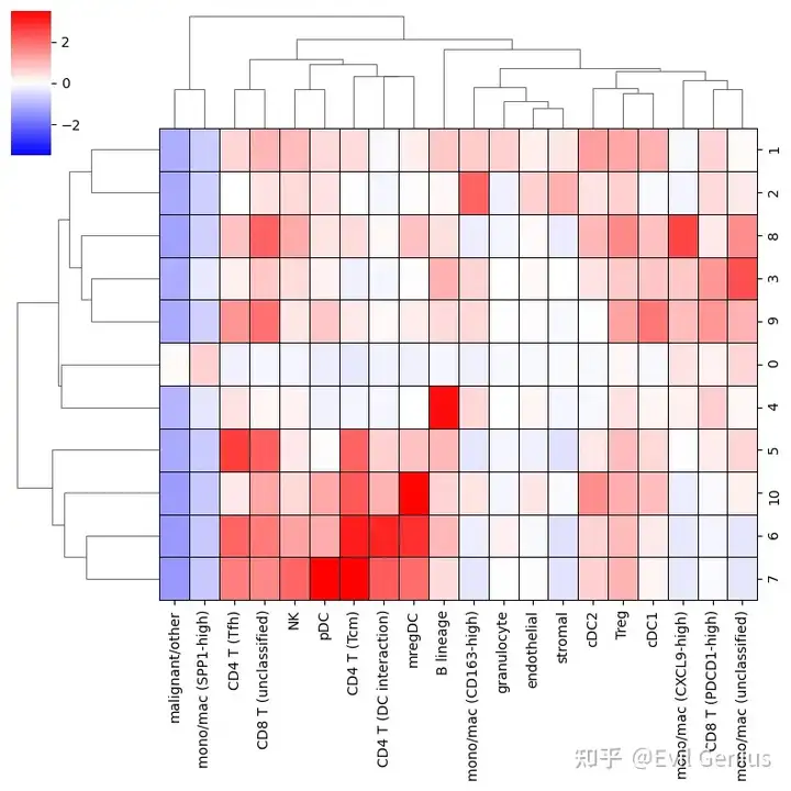
mb.plot.neighbors_profile_matrixplot(
    adata_neighbors,
    'niche',
    include_niches=[ # Exclude the miscellaneous niches from the plot
        niche
        for niche in set(adata_neighbors.obs['niche'])
        if niche != 'malignant/other'
    ],
    clustermap_kwargs={
        'linewidths': 0.5,
        'linecolor': 'black',
        'cmap': 'bwr',
        'clip_on': False,
        'vmin': -3.5,
        'vmax': 3.5,
        'figsize': (8,8)
    }
)
生活很好,有你更好
原创声明:本文系作者授权腾讯云开发者社区发表,未经许可,不得转载。
如有侵权,请联系 cloudcommunity@tencent.com 删除。
原创声明:本文系作者授权腾讯云开发者社区发表,未经许可,不得转载。
如有侵权,请联系 cloudcommunity@tencent.com 删除。
评论
登录后参与评论
推荐阅读
目录
腾讯云开发者

Copyright © 2013 - 2026 Tencent Cloud. All Rights Reserved. 腾讯云 版权所有
深圳市腾讯计算机系统有限公司 ICP备案/许可证号:粤B2-20090059 ![]() 粤公网安备44030502008569号
粤公网安备44030502008569号
腾讯云计算(北京)有限责任公司 京ICP证150476号 | 京ICP备11018762号