
线性回归图没有给我有意义的可视化
我正在使用一些时间序列的功耗数据,并试图对其进行线性回归分析。
数据有以下列:
日期,Denmark_consumption,Germany_consumption,Czech_consumption,Austria_consumption。
它是时间序列数据,频率为小时.
然而,每一列的值都是NaN的我的目标是创建一个线性回归模型,对没有空值的数据子集进行训练和测试,然后尝试预测丹麦消费列的值,例如,它目前有一个NaN值。
我计划使用一个国家消费栏以及序数值中的日期作为我的培训/测试功能,试图预测第二个国家的消费价值。
这里是数据的一个例子。
Date                   Denmark    Germany    Czech   Austria

2018-01-01 00:00:00     1607.0  42303.0     5520    6234.0

2018-01-01 01:00:00     1566.0  41108.0     5495    6060.0

2018-01-01 02:00:00     1460.0  40554.0     5461    5872.0

2018-01-01 03:00:00     1424.0  38533.0     5302    5564.0

2018-01-01 04:00:00     1380.0  38494.0     5258    5331.0
我做了几件事。
- 我删除了带有空值的行,以创建培训和测试数据集.
- I将date列设置为数据帧索引.
- I从每小时到每周对数据进行抽样。我使用了默认的“平均”聚合函数.
- I将日期作为一列添加到培训和测试数据中,并将其转换为序号值。
由于各种消费值都是高度相关的,所以我只对和X_test数据集使用了德国消费列。
我使用sklearn建立了一个线性回归模型,并以德国消费量和序号日期作为我的“X”和丹麦消费量作为我的“Y”对数据进行拟合。
我试图通过散点图和线来绘制输出,但是我得到了一个如下所示的图形:

为什么我的情节看上去像个涂鸦的人?我还以为会有一条单线呢。
下面是我的x_train数据集的一个示例
                        Germany    Date
                      consumption
Date
2018-07-08         44394.125000  736883
2019-01-16         66148.125000  737075
2019-08-03         45718.083333  737274
2019-06-09         41955.250000  737219
2020-03-04         61843.958333  737488
下面是我的y_train数据集的一个示例。
Date
2018-01-01    1511.083333
2018-01-02    1698.625000
2018-01-03    1781.291667
2018-01-04    1793.458333
2018-01-05    1796.875000
Name: Denmark_consumption, dtype: float64
这是实际的相关代码。
lin_model = LinearRegression()
lin_model.fit(X_train,y_train)
y_pred = lin_model.predict(X_test)
plt.scatter(X_test['Date'].map(dt.datetime.fromordinal),y_pred,color='black')
plt.plot(X_test['Date'],y_pred)
系数、R平方和均方误差为:
Coefficients:
 [0.01941453 0.01574128]
Mean squared error: 14735.12
Coefficient of determination: 0.51
有人能让我知道我做错了什么吗?另外,我的方法准确吗?尝试从第二个国家的消费+日期组合中预测消费价值是否有意义?
任何帮助都很感激。

回答 1
Stack Overflow用户
发布于 2020-07-22 20:35:05
你的方法很复杂,但可行。就我个人而言,我认为在德国的日期和德国的消费之间建立一个线性映射可能更容易,然后尝试用这种方式预测丹麦的消费量。
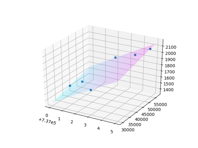
然而,坚持您的方法,您应该记住有两个自变量(德国的日期转换为整数,德国的消费)和丹麦的消费取决于这两个变量。因此,通过像现在这样,将测试日期与2D图中的预测相对应,您实际上忽略了消费变量。你应该策划的是德国的约会,德国的消费和丹麦在3D飞机上的消费。
另外,你也不应该期望得到一条线:用多元线性回归和两个自变量来预测一个平面。
这里是一个简单的例子,我把它放在一起,这与你可能想要达到的目标相似。随时根据需要更改日期的格式。
import pandas as pd
import numpy as np
import datetime as dt
from mpl_toolkits.mplot3d import *
import matplotlib.pyplot as plt
from matplotlib import cm
from sklearn.linear_model import LinearRegression

from pandas.plotting import register_matplotlib_converters
register_matplotlib_converters()

# starts 2018/11/02
df_germany = pd.DataFrame({
    'Germany consumption': [45000, 47000, 48000, 42000, 50000],
    'Date': [737000, 737001, 737002, 737003, 737004]})
df_germany_test = pd.DataFrame({
    'Germany consumption': [42050, 42000, 57000, 30000, 52000, 53000],
    'Date': [737000, 737001, 737002, 737003, 737004, 737005]})
df_denmark = pd.DataFrame({
    'Denmark consumption':  [1500, 1600, 1700, 1800, 2000]
    })

X_train = df_germany.to_numpy()
y_train = df_denmark['Denmark consumption']

# make X_test the same as X_train to make sure all points are on the plane
# X_test = df_germany

# make X_test slightly different
X_test = df_germany_test

lin_model = LinearRegression()
lin_model.fit(X_train,y_train)
y_pred = lin_model.predict(X_test)

fig = plt.figure()
ax = fig.gca(projection='3d')
# plt.hold(True)

x_surf=np.linspace(min(X_test['Date'].values), max(X_test['Date'].values), num=20)
y_surf=np.linspace(min(X_test['Germany consumption'].values), max(X_test['Germany consumption'].values), num=20)
x_surf, y_surf = np.meshgrid(x_surf, y_surf)
b0 = lin_model.intercept_
b1, b2 = lin_model.coef_
z_surf = b0+ b2*x_surf + b1*y_surf
ax.plot_surface(x_surf, y_surf, z_surf, cmap=cm.cool, alpha = 0.2)    # plot a 3d surface plot

ax.scatter(X_test['Date'].values, X_test['Germany consumption'].values, y_pred, alpha=1.0)
plt.show()
https://stackoverflow.com/questions/63045562
复制


腾讯云开发者

