【机器学习】ID3、C4.5、CART 算法


常见的决策树算法
1. ID3
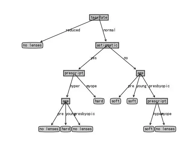
ID3(Iterative Dichotomiser 3)算法使用信息增益作为特征选择的标准。它是一种贪心算法,信息增益表示按某特征划分数据集前后信息熵的变化量,变化量越大,表示使用该特征划分的效果越好。但ID3偏向于选择取值较多的特征,可能导致过拟合。
以下是ID3算法的实现步骤:
1. 计算数据集的熵:熵是度量数据集无序程度的指标。 2. 计算每个属性的信息增益:信息增益是数据集的熵减去按照该属性分割后的条件熵。 3. 选择信息增益最大的属性:作为决策节点。 4. 分割数据集:根据选定的属性和它的值,将数据集分割成若干子集。 5. 递归构建决策树:对每个子集重复步骤1-4,直到所有数据都属于同一类别,或者已达到预设的最大深度。
以下是使用Python实现ID3算法的一个简单示例:
import numpy as np
import pandas as pd

# 计算熵
def calc_entropy(target_col):
    entropy = -np.sum([len(target_col[target_col == val]) / len(target_col) * np.log2(len(target_col[target_col == val]) / len(target_col))
                       for val in np.unique(target_col)])
    return entropy

# 按照给定属性分裂数据集
def split_dataset(dataset, index, value):
    return dataset[dataset.iloc[:, index] == value]

# 选择最好的数据集属性
def choose_best_feature_to_split(dataset):
    num_features = dataset.shape[1] - 1
    base_entropy = calc_entropy(dataset.iloc[:, -1])
    best_info_gain = 0.0
    best_feature = -1
    for i in range(num_features):
        feat_list = dataset.iloc[:, i]
        unique_vals = set(feat_list)
        new_entropy = 0.0
        for value in unique_vals:
            sub_dataset = split_dataset(dataset, i, value)
            prob = len(sub_dataset) / len(dataset)
            new_entropy += prob * calc_entropy(sub_dataset.iloc[:, -1])
        info_gain = base_entropy - new_entropy
        if info_gain > best_info_gain:
            best_info_gain = info_gain
            best_feature = i
    return best_feature

# 构建决策树
def create_tree(dataset, labels):
    # 检查数据集是否为空
    if len(dataset) == 0:
        return None
    # 检查数据集中的所有目标变量是否相同
    if len(set(dataset.iloc[:, -1])) <= 1:
        return dataset.iloc[0, -1]
    # 检查是否已达到最大深度或者没有更多的特征
    if len(dataset.columns) == 1 or len(set(dataset.iloc[:, -1])) == 1:
        return majority_cnt(dataset.iloc[:, -1])
    # 选择最好的数据集属性
    best_feat = choose_best_feature_to_split(dataset)
    best_feat_label = dataset.columns[best_feat]
    my_tree = {best_feat_label: {}}
    del(dataset[:, best_feat])
    unique_vals = set(dataset.iloc[:, -1])
    for value in unique_vals:
        sub_labels = best_feat_label + "_" + str(value)
        my_tree[best_feat_label][value] = create_tree(split_dataset(dataset, best_feat, value), sub_labels)
    return my_tree

# 找到出现次数最多的目标变量值
def majority_cnt(class_list):
    class_count = {}
    for vote in class_list:
        if vote not in class_count.keys():
            class_count[vote] = 1
        else:
            class_count[vote] += 1
    sorted_class_count = sorted(class_count.items(), key=lambda item: item[1], reverse=True)
    return sorted_class_count[0][0]

# 加载数据集
dataset = pd.read_csv("your_dataset.csv")  # 替换为你的数据集路径
labels = dataset.iloc[:, -1].name
dataset = dataset.iloc[:, 0:-1]  # 特征数据

# 创建决策树
my_tree = create_tree(dataset, labels)
print(my_tree)注:这个实现是为了教学目的而简化的,实际应用中通常会使用更高级的库和算法,如 scikit-learn 中的 DecisionTreeClassifier。
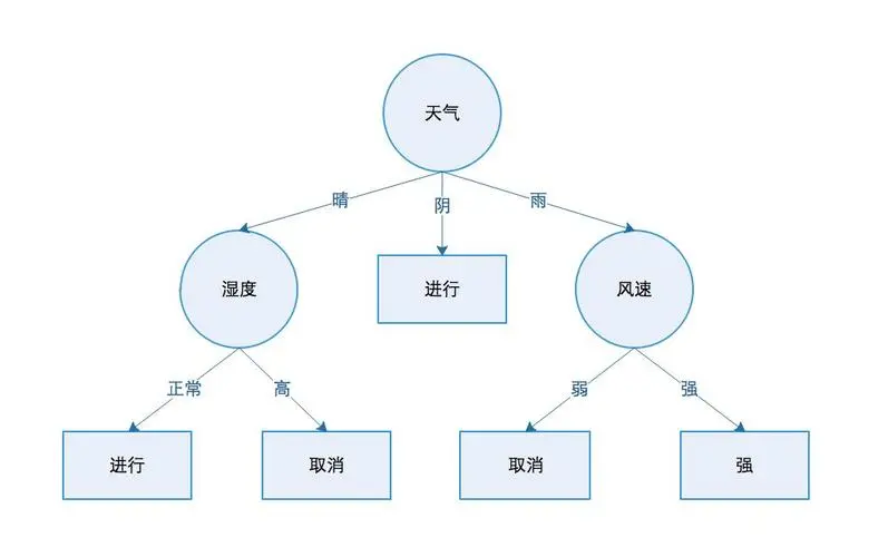
2. C4.5
C4.5是ID3的改进版,使用信息增益比替代信息增益作为特征选择标准,从而克服了ID3倾向于选择多值特征的缺点。此外,C4.5还能处理连续型特征和缺失值。
实现C4.5算法可以通过多种编程语言,但这里我将提供一个简化的Python实现,使用Python的基本库来构建决策树。这个实现将包括计算信息熵、信息增益、信息增益比,并基于这些度量来构建决策树。
1. 计算信息熵
信息熵是度量数据集无序程度的指标,计算公式为:
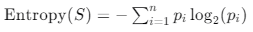
其中 pi 是第 i 个类别的样本在数据集中的比例。
2. 计算信息增益
信息增益是度量在知道特征 A 的条件下,数据集 S 的熵减少的程度。计算公式为:

其中 Sv 是特征 A 值为 v 时的子集。
3. 计算信息增益比
信息增益比是信息增益与特征 A 的固有信息的比值,计算公式为:
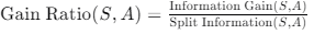
其中,分裂信息 Split Information(S, A) 是度量特征 A 的值分布的熵:

4. 构建决策树
使用以上计算方法,我们可以构建一个简单的C4.5决策树:
import numpy as np
import pandas as pd

def entropy(target_col):
    elements, counts = np.unique(target_col, return_counts=True)
    probabilities = counts / counts.sum()
    return -np.sum(probabilities * np.log2(probabilities))

def information_gain(data, feature, target):
    total_entropy = entropy(data[target])
    values = data[feature].unique()
    weighted_entropy = 0.0
    for value in values:
        sub_data = data[data[feature] == value]
        weighted_entropy += (len(sub_data) / len(data)) * entropy(sub_data[target])
    return total_entropy - weighted_entropy

def gain_ratio(data, feature, target):
    ig = information_gain(data, feature, target)
    split_info = entropy(data[feature])
    return ig / split_info if split_info != 0 else 0

def choose_best_feature_to_split(data, features, target):
    best_feature = None
    max_gain_ratio = -1
    for feature in features:
        gain_ratio_value = gain_ratio(data, feature, target)
        if gain_ratio_value > max_gain_ratio:
            max_gain_ratio = gain_ratio_value
            best_feature = feature
    return best_feature

def c45(data, features, target, tree=None, depth=0):
    if len(data[target].unique()) == 1:
        return data[target].mode()[0]

    if depth == 0:
        depth = 0
    elif depth > 10:  # Limit the depth to avoid overfitting
        return data[target].mode()[0]

    best_feat = choose_best_feature_to_split(data, features, target)
    if best_feat is None:
        return data[target].mode()[0]

    if len(data[best_feat].unique()) == 1:
        return data[target].mode()[0]

    tree = tree if tree else {best_feat: {}}
    unique_vals = data[best_feat].unique()

    for value in unique_vals:
        subtree = c45(data[data[best_feat] == value], features, target, tree=tree, depth=depth+1)
        tree[best_feat][value] = subtree
    return tree

# Example usage
data = pd.DataFrame({
    'Outlook': ['Sunny', 'Sunny', 'Overcast', 'Rain', 'Rain', 'Rain', 'Overcast', 'Sunny', 'Sunny', 'Rain', 'Sunny', 'Overcast', 'Overcast', 'Rain'],
    'Temperature': ['Hot', 'Hot', 'Hot', 'Mild', 'Cool', 'Cool', 'Cool', 'Mild', 'Cool', 'Mild', 'Mild', 'Mild', 'Hot', 'Mild'],
    'Humidity': ['High', 'High', 'High', 'High', 'Normal', 'Normal', 'Normal', 'High', 'Normal', 'Normal', 'Normal', 'High', 'Normal', 'High'],
    'Wind': ['Weak', 'Strong', 'Weak', 'Weak', 'Weak', 'Strong', 'Strong', 'Weak', 'Weak', 'Weak', 'Strong', 'Strong', 'Weak', 'Strong'],
    'PlayTennis': ['No', 'No', 'Yes', 'Yes', 'Yes', 'No', 'Yes', 'No', 'Yes', 'Yes', 'Yes', 'Yes', 'Yes', 'No']
})

features = ['Outlook', 'Temperature', 'Humidity', 'Wind']
target = 'PlayTennis'

tree = c45(data, features, target)
print(tree)注:这个实现是一个简化版,没有包括剪枝和处理连续变量的步骤。在实际应用中,你可能需要使用更复杂的数据结构和算法来优化性能和处理更复杂的情况。
3. CART
CART(分类与回归树)是一种既能用于分类也能用于回归的决策树算法。对于分类问题,CART使用基尼不纯度作为特征选择标准;对于回归问题,则使用方差作为分裂标准。CART构建的是二叉树,每个内部节点都是二元分裂。
以下是CART算法的基本步骤:
1. 选择最佳分割特征和分割点:使用基尼不纯度(Gini impurity)或均方误差(Mean Squared Error, MSE)作为分割标准,选择能够最大程度降低不纯度的特征和分割点。
2. 分割数据集:根据选定的特征和分割点,将数据集分割成两个子集。
3. 递归构建:对每个子集重复步骤1和2,直到满足停止条件(如达到最大深度、节点中的样本数量低于阈值或无法进一步降低不纯度)。
4. 剪枝:通过剪掉树的某些部分来简化树,以防止过拟合。
以下是一个简化的Python实现CART算法,使用基尼不纯度作为分割标准:
import numpy as np
import pandas as pd

def gini_impurity(y):
    class_probabilities = y.mean(axis=0)
    return 1 - np.sum(class_probabilities ** 2)

def best_split(data, target_column, features):
    best_feature = None
    best_threshold = None
    best_gini = float('inf')

    for feature in features:
        for idx in np.unique(data[feature]):
            threshold = (data[feature] < idx).mean()
            split_data = data[data[feature] < idx]
            gini = (len(data) - len(split_data)) / len(data) * gini_impurity(split_data[target_column]) + \
                   len(split_data) / len(data) * gini_impurity(data[(data[target_column] == target_column.mode())[data[target_column] >= idx]][target_column])
            if gini < best_gini:
                best_gini = gini
                best_feature = feature
                best_threshold = threshold

    return best_feature, best_threshold

def build_tree(data, target_column, features, depth=0, max_depth=None):
    if max_depth is None:
        max_depth = np.inf
    if len(data[target_column].unique()) == 1 or len(data) == 1 or depth >= max_depth:
        return data[target_column].mode()[0]

    best_feature, best_threshold = best_split(data, target_column, features)
    tree = {best_feature: {}}
    features = [f for f in features if f != best_feature]

    split_function = lambda x: x[best_feature] < best_threshold
    left_indices = np.array([bool(split_function(row)) for row in data.itertuples()])
    right_indices = np.array([not bool(split_function(row)) for row in data.itertuples()])

    left_data = data[left_indices]
    right_data = data[right_indices]

    if not left_data.empty:
        tree[best_feature][0] = build_tree(left_data, target_column, features, depth+1, max_depth)
    if not right_data.empty:
        tree[best_feature][1] = build_tree(right_data, target_column, features, depth+1, max_depth)

    return tree

# Example usage
data = pd.DataFrame({
    'Feature1': [1, 2, 4, 6, 8, 10],
    'Feature2': [2, 4, 6, 8, 10, 12],
    'Target': ['Yes', 'No', 'Yes', 'No', 'Yes', 'No']
})

features = ['Feature1', 'Feature2']
target_column = 'Target'

tree = build_tree(data, target_column, features)
print(tree)注:这个实现是一个简化的版本,没有包括剪枝步骤。在实际应用中,你可能需要使用更复杂的数据结构和算法来优化性能和处理更复杂的情况。此外,对于回归问题,需要使用均方误差(MSE)而不是基尼不纯度作为分割标准。
在实践中,通常会使用像scikit-learn这样的机器学习库来构建CART树,因为它们提供了更高效和更可靠的实现。例如,scikit-learn中的DecisionTreeClassifier和DecisionTreeRegressor类实现了CART算法。
决策树的优缺点 优点: - 易于理解和解释。 - 可以处理数值和类别数据。 - 不需要数据标准化。 - 可以可视化。 缺点: - 容易过拟合。 - 对于某些数据集,构建的树可能非常大。 - 对于缺失数据敏感。 决策树的优化 - 剪枝:通过减少树的大小来减少过拟合。 - 集成方法:如随机森林和梯度提升树,可以提高模型的泛化能力。
执笔至此,感触彼多,全文将至,落笔为终,感谢各位读者的支持,如果对你有所帮助,还请一键三连支持我,我会持续更新创作。
本文参与 腾讯云自媒体同步曝光计划,分享自作者个人站点/博客。
原始发表:2024-09-28,如有侵权请联系 cloudcommunity@tencent.com 删除
评论
登录后参与评论
推荐阅读
目录
腾讯云开发者

Copyright © 2013 - 2026 Tencent Cloud. All Rights Reserved. 腾讯云 版权所有
深圳市腾讯计算机系统有限公司 ICP备案/许可证号:粤B2-20090059 ![]() 粤公网安备44030502008569号
粤公网安备44030502008569号
腾讯云计算(北京)有限责任公司 京ICP证150476号 | 京ICP备11018762号