9种神经网络优化算法详解
原创

公众号:尤而小屋 编辑:Peter 作者:Peter
大家好,我是Peter~
在深度学习中,有一个“损失loss”的概念,它告诉我们:模型在训练数据中表现的“多差”。
现在,我们需要利用这个损失来训练我们的网络,使其表现得更好。本质上,我们需要做的是利用损失并尝试将其最小化,因为较低的损失意味着我们的模型将会表现得更好。最小化(或最大化)任何数学表达式的这个过程被称为优化。
理解全局最小化和局部最小化
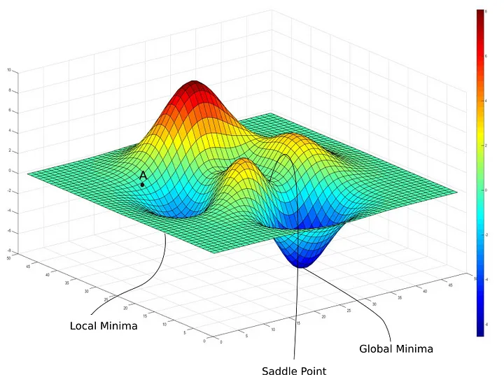
- 局部最小化:Local Minima
- 全局最小化:Global Minima
优化器如何工作
优化器是用于改变神经网络属性(例如权重和学习率)的算法或方法,以减少损失。优化器通过最小化函数来解决优化问题。
为了更好地理解优化器的作用,可以想象一个蒙着眼睛的登山者试图走下一座山。无法确切知道他该往哪个方向走,但他能判断自己是在下山(取得进展)还是在上山(失去进展)。只要他一直朝着下山的方向前进,最终就能到达山脚。
正在上传图片...
同样,在训练神经网络时,我们无法从一开始就确定模型的权重应该是什么,但可以通过基于损失函数的不断调整(类似于判断登山者是否在下山)来逐步接近目标。
优化器的作用就在于此: 它决定了如何调整神经网络的权重和学习率以减少损失。优化算法通过不断优化损失函数,帮助模型尽可能地输出准确的结果。
9种优化器
列举9种不同类型的优化器以及它们是如何精确地工作以最小化损失函数的。
- Gradient Descent
- Stochastic Gradient Descent, SGD
- Mini-Batch Stochastic Gradient Descent, MB-SGD
- SGD with Momentum
- Nesterov Accelerated Gradient, NAG
- Adaptive Gradient, AdaGrad
- AdaDelta
- RMSprop
- Adam
梯度下降Gradient Descent
基本思想
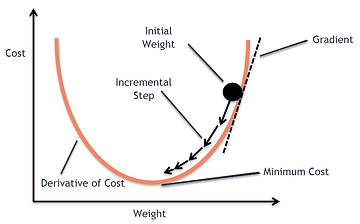
梯度下降(Gradient Descent)是一种优化算法,用于寻找可微函数的局部最小值。其目标是通过迭代调整模型参数,最小化代价函数(Cost Function)。以下是梯度下降算法的基本思想:
- 目标:找到模型参数的最优值,使得代价函数达到最小值。
- 方法:利用函数的梯度(即导数)来确定参数调整的方向。梯度(Gradient)指的是函数在某一点的梯度是一个向量,指向函数增长最快的方向。
到底什么是梯度?
"A gradient measures how much the output of a function changes if you change the inputs a little bit." — Lex Fridman (MIT)
梯度下降的核心思想是:沿着梯度的反方向(即函数下降最快的方向)调整参数。
算法步骤
- 初始化参数:
- 选择初始参数值(通常随机初始化或使用特定策略)。
- 设置学习率(Learning Rate),学习率决定了每次迭代中参数更新的步长。
- 计算梯度: 计算代价函数对每个参数的偏导数,得到梯度向量。
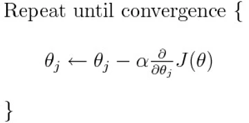
- 更新参数: 使用梯度下降更新公式调整参数: $$
\theta = \theta - \alpha \cdot \nabla J(\theta)
$$
其中:
- $\theta\$ 是模型参数。
- $\alpha\$ 是学习率。
- $\nabla J(\theta)$ 是代价函数 $J(\theta)\$ 对参数 $\theta\$ 的梯度。
重复计算梯度和更新参数的过程,直到满足终止条件(如收敛或达到最大迭代次数)。
收敛条件
- 收敛判断:当代价函数的变化量小于某个阈值,或梯度的范数小于某个阈值时,认为算法收敛。
- 停止条件:可以设置最大迭代次数,防止算法陷入无限循环。
学习率的作用
- 学习率的选择:
- 如果学习率过大,可能导致参数更新过度,使代价函数无法收敛甚至发散。
- 如果学习率过小,会使收敛速度过慢,增加训练时间。
- 动态调整学习率:在训练过程中,可以采用动态调整学习率的策略,如学习率衰减(Learning Rate Decay),以加速收敛。
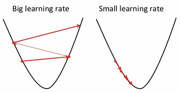
通过图像的形式描述不同学习率的过程:
可以看到学习率不能过大或过小。
for i in range(nb_epochs):
    params_grad = evaluate_gradient(loss_function, data, params)
    params = params - learning_rate * params_grad
优缺点
Advantages:
- 计算简单
- 实现容易
- 容易理解
Disadvantages:
- 可能陷入局部最小值。
- 权重是在计算整个数据集的梯度之后才更新的。因此,如果数据集太大,可能需要花费较长时间才能收敛到最小值。
- 需要大量内存来计算整个数据集的梯度。
案例
线性回归+梯度下降:
import numpy as np
import matplotlib.pyplot as plt

# 生成模拟数据
np.random.seed(0)
X = 2 * np.random.rand(100, 1)  # 100个随机数据点
y = 4 + 3 * X + np.random.randn(100, 1)  #  y = 4 + 3x + 噪声

# 添加偏置项
X_b = np.c_[np.ones((100, 1)), X]  # 在X中添加一列1,作为偏置项

# 初始化参数
w = np.random.randn(2, 1)  # 随机初始化参数w和b
learning_rate = 0.01  # 学习率
n_iterations = 1000  # 迭代次数

# 梯度下降
for iteration in range(n_iterations):
    y_pred = X_b.dot(w)  # 计算预测值
    gradients = 2 / len(X_b) * X_b.T.dot(y_pred - y)  # 计算梯度
    w = w - learning_rate * gradients  # 更新参数

    # 每隔一定次数打印损失
    if iteration % 100 == 0:
        loss = np.mean((y_pred - y) ** 2)
        print(f"Iteration {iteration}: Loss = {loss}")

# 打印最终结果
print(f"Optimal parameters: w = {w[1][0]}, b = {w[0][0]}")

# 可视化结果
plt.scatter(X, y, color='blue', label='Data points')
plt.plot(X, X_b.dot(w), color='red', label='Fitted line')
plt.xlabel('X')
plt.ylabel('y')
plt.legend()
plt.show()
每100次输出一次Loss值:
Iteration 0: Loss = 82.6630580098186
Iteration 100: Loss = 1.03474536503957
Iteration 200: Loss = 1.0053717575274455
Iteration 300: Loss = 0.9992232039352024
Iteration 400: Loss = 0.9959987975896929
Iteration 500: Loss = 0.9943068126783625
Iteration 600: Loss = 0.9934189550799246
Iteration 700: Loss = 0.9929530578311317
Iteration 800: Loss = 0.9927085814119238
Iteration 900: Loss = 0.992580294070233
Optimal parameters: w = 2.9827303563323175, b = 4.20607718142562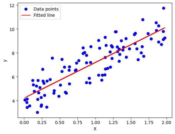
随机梯度下降Stochastic Gradient Descent (SGD)
定义
随机梯度下降(SGD)是一种优化算法,用于在训练机器学习模型时最小化损失函数。它是梯度下降算法的一种扩展,通过每次只使用一个训练样本(或少量样本)来计算梯度,从而减少计算量和内存需求。
基本思想
目标:通过迭代更新模型参数,最小化损失函数 J(θ)。
方法:每次只使用一个训练样本 (x(i),y(i)) 来计算梯度,并更新参数。
在SGD算法中,每次只取一个数据点来计算导数。
SGD(随机梯度下降)针对每个训练样本 x(i) 和对应的标签 y(i) 进行参数更新。
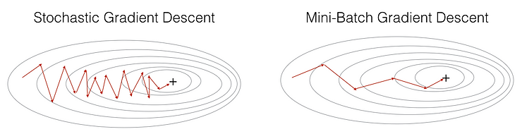
θ = θ − α⋅∂(J(θ;x(i),y(i)))/∂θ对比随机梯度下降SGD和梯度下降GD:
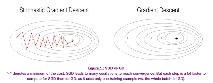
在左边,随机梯度下降(SGD,其中每步 m=1)为每个样本进行一次梯度下降步骤;而在右边是完整的梯度下降(每整个训练集进行1次步骤)。
观察结果表明,在SGD中,更新需要比梯度下降更多的迭代次数才能到达最小值。在右边,梯度下降到达最小值的步数更少,但SGD算法更“嘈杂”,需要更多的迭代次数。
在TensorFlow中的使用:
from tensorflow.keras.optimizers import SGD
optimizer = SGD(learning_rate=0.01, momentum=0.0, nesterov=False
算法步骤
- 初始化参数:
- 随机初始化模型参数 θ。
- 设置学习率 α。
- 迭代更新:
- 对于每个训练样本 (x(i),y(i)):
- 计算损失函数 J(θ) 关于参数 θ 的梯度 ∇J(θ)。
- 更新参数:
- θ=θ−α⋅∇J(θ)
- 重复步骤:
重复上述过程,直到满足终止条件(如收敛或达到最大迭代次数)。
SGD的代码片段只是在训练样本上增加了一个循环,并针对每个样本计算梯度。
for i in range(nb_epochs):
    np.random.shuffle(data)
    for example in data:
        params_grad = evaluate_gradient(loss_function, example, params)
        params = params - learning_rate * params_grad
优缺点
Advantages:
- 计算效率高:每次只处理一个样本,计算量小,适合大规模数据集。
- 内存需求低:不需要一次性加载整个数据集,节省内存。
- 实时更新:参数在每个样本后更新,能够快速响应数据的变化。
Disadvantages:
- 噪声大:每次更新基于单个样本,梯度估计可能不准确,导致更新过程“嘈杂”。
- 收敛速度慢:可能需要更多迭代次数才能收敛到最小值。
- 易陷入局部最小值:由于更新的随机性,可能在局部最小值附近徘徊。
随机梯度下降(SGD)通过每次只处理一个样本,减少了计算量和内存需求,同时保持了快速的参数更新能力。
虽然存在一定的噪声和收敛速度较慢的问题,但通过适当的调整学习率和优化策略,SGD在许多实际应用中表现出色。
案例
线性回归+随机梯度下降:
import numpy as np
import matplotlib.pyplot as plt

np.random.seed(0)
X = 2 * np.random.rand(100, 1)  # 生成100个随机数据点
y = 4 + 3 * X + np.random.randn(100, 1)  # 真实关系 y = 4 + 3x + 噪声

# 偏置
X_b = np.c_[np.ones((100, 1)), X]  # 在X中添加一列1,作为偏置项

# 初始化参数
w = np.random.randn(2, 1)  # 随机初始化参数w和b
learning_rate = 0.01  # 学习率
n_iterations = 1000  # 迭代次数
m = len(X_b)  # 样本数量

# 随机梯度下降
for iteration in range(n_iterations):
    # 重点:随机选择一个样本
    random_index = np.random.randint(m)
    xi = X_b[random_index:random_index + 1]
    yi = y[random_index:random_index + 1]

    # 计算梯度
    gradients = 2 * xi.T.dot(xi.dot(w) - yi)
    # 更新参数
    w = w - learning_rate * gradients

    # 每隔100次数打印损失
    if iteration % 100 == 0:
        y_pred = X_b.dot(w)
        loss = np.mean((y_pred - y) ** 2)
        print(f"Iteration {iteration}: Loss = {loss}")

print(f"Optimal parameters: w = {w[1][0]}, b = {w[0][0]}")

plt.scatter(X, y, color='blue', label='Data points')
plt.plot(X, X_b.dot(w), color='red', label='Fitted line')
plt.xlabel('X')
plt.ylabel('y')
plt.legend()
plt.show()

# 结果
Iteration 0: Loss = 69.02554947814826
Iteration 100: Loss = 1.0436708721159689
Iteration 200: Loss = 1.041294923577367
Iteration 300: Loss = 1.010387875806174
Iteration 400: Loss = 1.0070132665208844
Iteration 500: Loss = 1.091486693566191
Iteration 600: Loss = 0.9986328028787116
Iteration 700: Loss = 1.0340118681106303
Iteration 800: Loss = 0.9984103484305885
Iteration 900: Loss = 1.0082506511215945
Optimal parameters: w = 3.052173302887621, b = 4.352670551847081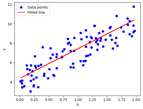
小批量随机梯度下降(Mini Batch Stochastic Gradient Descent, MB-SGD)
小批量随机梯度下降(Mini Batch Stochastic Gradient Descent, MB-SGD)是梯度下降算法的一种改进,结合了批量梯度下降(Batch Gradient Descent)和随机梯度下降(Stochastic Gradient Descent, SGD)的优点。
它通过每次使用一个小批量(Mini-Batch)的数据来计算梯度,从而在计算效率和稳定性之间取得平衡。
基本思想
目标:通过迭代更新模型参数,最小化损失函数 J(θ)。
方法:每次从训练集中随机抽取一个小批量的数据(通常包含几十个样本),计算该小批量数据的梯度,并更新参数。
算法步骤
- 初始化参数:
- 随机初始化模型参数θ。
- 设置学习率α。
- 定义小批量的大小m(通常为2的幂,如32、64、128等)。
- 划分数据集:
将整个训练集划分为若干个小批量,每个小批量包含 m 个样本。
- 迭代更新: $$ \nabla J(\theta) = \frac{1}{m} \sum_{i=1}^{m} \nabla J(\theta; x^{(i)}, y^{(i)}) $$
- 更新参数: $$ \theta = \theta - \alpha \cdot \nabla J(\theta) $$ 重复步骤: 重复上述过程,直到满足终止条件(如收敛或达到最大迭代次数)。
使用mini-batches参数:
for i in range(nb_epochs):
    np.random.shuffle(data)
    for batch in get_batches(data, batch_size=50):
        params_grad = evaluate_gradient(loss_function, batch, params)
        params = params - learning_rate * params_grad
Advantages:
- 相比于标准的随机梯度下降(SGD)算法,收敛的时间复杂度更低。
Disadvantages::
- 与梯度下降(GD)算法相比,小批量随机梯度下降(MB-SGD)的更新过程更加“嘈杂”。
- 比梯度下降(GD)算法需要更长时间才能收敛。
- 可能会陷入局部最小值。
案例
逻辑回归+小批量随机梯度下降:
import numpy as np
import matplotlib.pyplot as plt

# 生成一些简单的二分类数据
np.random.seed(42)
X = np.random.randn(100, 2)  # 100个样本,每个样本有2个特征
y = (X[:, 0] + X[:, 1] > 0).astype(int)  # 标签,根据两个特征之和是否大于0来分类

# 添加偏置项
X_b = np.c_[np.ones((100, 1)), X]

# 初始化参数
theta = np.random.randn(3)

# 定义sigmoid函数
def sigmoid(z):
    return 1 / (1 + np.exp(-z))

# 小批量随机梯度下降
def mini_batch_gradient_descent(X, y, theta, learning_rate=0.01, batch_size=10, epochs=100):
    m = len(y)
    for epoch in range(epochs):
        indices = np.random.permutation(m)
        X_shuffled = X[indices]
        y_shuffled = y[indices]
        for i in range(0, m, batch_size):
            xi = X_shuffled[i:i+batch_size]
            yi = y_shuffled[i:i+batch_size]
            gradients = xi.T.dot(sigmoid(xi.dot(theta)) - yi) / len(yi)
            theta -= learning_rate * gradients
        if epoch % 10 == 0:
            loss = -np.mean(yi * np.log(sigmoid(xi.dot(theta))) + (1 - yi) * np.log(1 - sigmoid(xi.dot(theta))))
            print(f'Epoch {epoch}, Loss: {loss}')
    return theta

# 训练模型
learning_rate = 0.1
batch_size = 10
epochs = 100
theta = mini_batch_gradient_descent(X_b, y, theta, learning_rate, batch_size, epochs)

print("Trained parameters:", theta)

# 预测函数
def predict(X, theta):
    probabilities = sigmoid(X.dot(theta))
    return probabilities >= 0.5

# 测试模型
predictions = predict(X_b, theta)
accuracy = np.mean(predictions == y)
print(f"Accuracy: {accuracy * 100:.2f}%")

# 可视化模型和预测效果
def plot_decision_boundary(X, y, theta):
    plt.figure(figsize=(10, 6))
    plt.scatter(X[:, 1], X[:, 2], c=y, marker='o', cmap='winter')
    x1_min, x1_max = X[:, 1].min() - 1, X[:, 1].max() + 1
    x2_min, x2_max = X[:, 2].min() - 1, X[:, 2].max() + 1
    xx1, xx2 = np.meshgrid(np.linspace(x1_min, x1_max, 100), np.linspace(x2_min, x2_max, 100))
    grid = np.c_[np.ones((xx1.ravel().shape[0], 1)), xx1.ravel(), xx2.ravel()]
    Z = sigmoid(grid.dot(theta)).reshape(xx1.shape)
    plt.contourf(xx1, xx2, Z, alpha=0.3, cmap='winter')
    plt.xlabel('Feature 1')
    plt.ylabel('Feature 2')
    plt.title('Decision Boundary and Data Points')
    plt.show()

# 调用绘图函数
plot_decision_boundary(X_b, y, theta)

# 结果
Epoch 0, Loss: 0.424476004585312
Epoch 10, Loss: 0.2950600705690528
Epoch 20, Loss: 0.19517955198064607
Epoch 30, Loss: 0.07305972705615815
Epoch 40, Loss: 0.15634434000393793
Epoch 50, Loss: 0.09763985480946141
Epoch 60, Loss: 0.22901934823973308
Epoch 70, Loss: 0.06952644778550963
Epoch 80, Loss: 0.12401363486230814
Epoch 90, Loss: 0.05268405861771795
Trained parameters: [-0.17306619  3.80492488  3.80846526]
Accuracy: 99.00%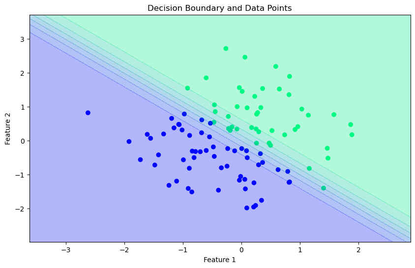
SGD with Momentum
基本原理
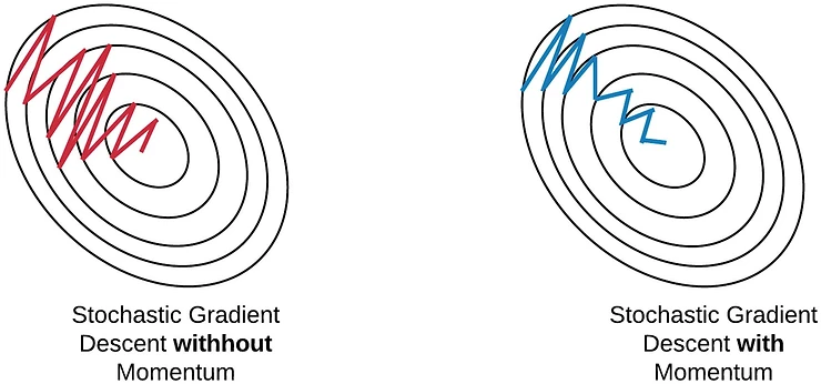
小批量随机梯度下降(MB-SGD)算法的一个主要缺点是权重更新非常“嘈杂”。带动量的随机梯度下降(SGD with Momentum)通过降噪梯度克服了这一缺点,它在传统的随机梯度下降(SGD)的基础上引入了动量Momentum机制,在每次更新时,通过考虑历史梯度信息来加速收敛并减少噪声。
算法步骤
- 初始化参数
- 随机初始化模型参数 $\theta$
- 初始化动量参数 v (通常初始化为零向量)。
- 设置学习率 $\alpha$ 和动量系数$\gamma $(通常取值为0.9或0.99)。
- 迭代更新
- 对于每个训练样本$(x^{(i)}, y^{(i)}) $ 或小批量数据: 1. 计算当前梯度$\nabla J(\theta)$: $$ \nabla J(\theta) = \frac{\partial J(\theta; x^{(i)}, y^{(i)})}{\partial \theta} $$ 2. 更新动量参数 $ v $: $$ v = \gamma \cdot v - \alpha \cdot \nabla J(\theta) $$ 其中: - $\gamma\$ 是动量系数,控制历史梯度的衰减速度。 - $\alpha\$ 是学习率,控制更新步长。 1. 更新参数$ \theta $: $$ \theta = \theta + v $$
- 重复步骤
- 重复上述过程,直到满足终止条件(如收敛或达到最大迭代次数)。
优缺点
Advantages:
- 减少噪声:通过考虑历史梯度信息,减少了更新过程中的噪声。
- 加速收敛:动量机制帮助模型更快地收敛到最小值,特别是在损失函数的“山谷”中。
- 减少振荡:在接近最小值时,动量机制可以减少参数更新的振荡。
Disadvantages:
- 超参数选择:需要选择合适的动量系数 $\gamma\$ 和学习率 $\alpha$,这可能需要一些实验和调整。
- 计算复杂度:虽然每次更新的计算量与SGD相当,但引入动量机制会增加一些额外的计算开销。
在TensorFlow中的使用:
from tensorflow.keras.optimizers import SGD
optimizer = SGD(learning_rate=0.01, momentum=0.9, nesterov=False)
案例
import numpy as np
import matplotlib.pyplot as plt

# 生成一些随机数据
np.random.seed(42)
X = np.random.randn(200, 2)
y = np.logical_xor(X[:, 0] > 0, X[:, 1] > 0)
y = y.astype(int)

# 定义激活函数和其导数
def sigmoid(x):
    return 1 / (1 + np.exp(-x))

def sigmoid_derivative(x):
    return x * (1 - x)

# 定义网络结构
input_size = 2
hidden_size = 4
output_size = 1

# 初始化参数
W1 = np.random.randn(input_size, hidden_size)
b1 = np.zeros((1, hidden_size))
W2 = np.random.randn(hidden_size, output_size)
b2 = np.zeros((1, output_size))

# 超参数
learning_rate = 0.01
momentum = 0.9
n_iterations = 10000

# 动量初始化
velocity_W1 = np.zeros_like(W1)
velocity_b1 = np.zeros_like(b1)
velocity_W2 = np.zeros_like(W2)
velocity_b2 = np.zeros_like(b2)

# SGD with Momentum
for iteration in range(n_iterations):
    # 前向传播
    hidden_input = np.dot(X, W1) + b1
    hidden_output = sigmoid(hidden_input)
    output_input = np.dot(hidden_output, W2) + b2
    output = sigmoid(output_input)

    # 计算损失
    loss = np.mean((output - y.reshape(-1, 1)) ** 2)

    # 反向传播
    d_output = (output - y.reshape(-1, 1)) * sigmoid_derivative(output)
    d_hidden = np.dot(d_output, W2.T) * sigmoid_derivative(hidden_output)

    # 计算梯度
    dW2 = np.dot(hidden_output.T, d_output)
    db2 = np.sum(d_output, axis=0, keepdims=True)
    dW1 = np.dot(X.T, d_hidden)
    db1 = np.sum(d_hidden, axis=0, keepdims=True)

    # 更新动量
    velocity_W2 = momentum * velocity_W2 + learning_rate * dW2
    velocity_b2 = momentum * velocity_b2 + learning_rate * db2
    velocity_W1 = momentum * velocity_W1 + learning_rate * dW1
    velocity_b1 = momentum * velocity_b1 + learning_rate * db1

    # 更新参数
    W2 = W2 - velocity_W2
    b2 = b2 - velocity_b2
    W1 = W1 - velocity_W1
    b1 = b1 - velocity_b1

    # 打印损失
    if iteration % 1000 == 0:
        print(f"Iteration {iteration}, Loss: {loss}")

# 绘制决策边界
def plot_decision_boundary(X, y, model):
    x_min, x_max = X[:, 0].min() - 1, X[:, 0].max() + 1
    y_min, y_max = X[:, 1].min() - 1, X[:, 1].max() + 1
    xx, yy = np.meshgrid(np.arange(x_min, x_max, 0.01),
                         np.arange(y_min, y_max, 0.01))
    Z = model(np.c_[xx.ravel(), yy.ravel()])
    Z = Z.reshape(xx.shape)
    plt.contourf(xx, yy, Z, alpha=0.8)
    plt.scatter(X[:, 0], X[:, 1], c=y, edgecolors='k', marker='o')
    plt.xlabel("X1")
    plt.ylabel("X2")
    plt.title("Decision Boundary")
    plt.show()

# 定义模型预测函数
def predict(X):
    hidden_input = np.dot(X, W1) + b1
    hidden_output = sigmoid(hidden_input)
    output_input = np.dot(hidden_output, W2) + b2
    output = sigmoid(output_input)
    return (output > 0.5).astype(int)

# 绘制决策边界
plot_decision_boundary(X, y, predict)

# 结果
Iteration 0, Loss: 0.24866396311697422
Iteration 1000, Loss: 0.059649335744367704
Iteration 2000, Loss: 0.05161391737798015
Iteration 3000, Loss: 0.047237416656551276
Iteration 4000, Loss: 0.043973210315089856
Iteration 5000, Loss: 0.041256973919964544
Iteration 6000, Loss: 0.03895073389030161
Iteration 7000, Loss: 0.037002859681704706
Iteration 8000, Loss: 0.035360650108840486
Iteration 9000, Loss: 0.03396667708959878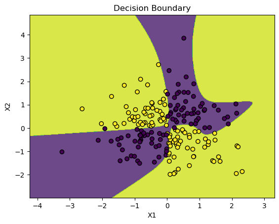
Nesterov Accelerated Gradient, NAG
基本原理
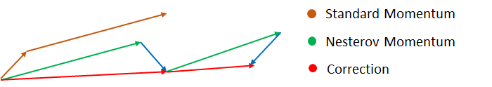
动量法每下降一步都是由前面下降方向的一个累积和当前点的梯度方向组合而成。于是一位大神(Nesterov)就开始思考,既然每一步都要将两个梯度方向(历史梯度、当前梯度)做一个合并再下降,那为什么不先按照历史梯度往前走那么一小步,按照前面一小步位置的“超前梯度”来做梯度合并呢?
如此一来,小球就可以先不管三七二十一先往前走一步,在靠前一点的位置看到梯度,然后按照那个位置再来修正这一步的梯度方向。如此一来,有了超前的眼光,小球就会更加”聪明“, 这种方法被命名为Nesterov accelerated gradient 简称 NAG
Nesterov Accelerated Gradient(NAG)是一种改进的梯度下降优化算法,它在传统的动量优化算法的基础上引入了“前瞻性”更新机制,从而提高了收敛速度并减少了震荡。
NAG的核心思想是在计算梯度时:
- 先根据之前的动量方向进行一个预期的更新
- 然后再根据这个预期位置计算梯度。
这种方法使得参数更新更加“前瞻”,避免了传统动量方法中可能出现的过冲问题。
数学公式
记$vt$为第t次迭代梯度的累积:
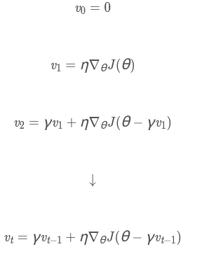
- 初始化:$ v_0 = 0 $
- 第一次迭代: $v1 = \eta \nabla\theta J(\theta) $
- 第二次迭代:$ v2 = \gamma v_1 + \eta \nabla\theta J(\theta - \gamma v_1) $
- 一般迭代规则(第 ( t ) 次迭代):$ vt = \gamma v{t-1} + \eta \nabla\theta J(\theta - \gamma v{t-1}) $
其中:
- $ \eta $ 是学习率
- $ \gamma $ 是动量系数
- $ \nabla_\theta J(\theta) $是损失函数$J$关于参数$ \theta $的梯度
在TensorFlow中的使用:
from tensorflow.keras.optimizers import SGD
optimizer = SGD(learning_rate=0.01, momentum=0.9, nesterov=True)
案例
import numpy as np
import matplotlib.pyplot as plt
class LogisticRegressionNAG:
def __init__(self, learning_rate=0.01, momentum=0.9, n_iters=1000):
self.learning_rate = learning_rate
self.momentum = momentum
self.n_iters = n_iters
self.weights = None
self.bias = None
self.v_w = None
self.v_b = None
def sigmoid(self, z):
return 1 / (1 + np.exp(-z))
def fit(self, X, y):
n_samples, n_features = X.shape
self.weights = np.zeros(n_features)
self.bias = 0
self.v_w = np.zeros(n_features)
self.v_b = 0
losses = [] # 用于记录损失值
for _ in range(self.n_iters):
# 临时更新
temp_weights = self.weights - self.momentum * self.v_w
temp_bias = self.bias - self.momentum * self.v_b
# 计算梯度
linear_model = np.dot(X, temp_weights) + temp_bias
y_pred = self.sigmoid(linear_model)
dw = (1 / n_samples) * np.dot(X.T, (y_pred - y))
db = (1 / n_samples) * np.sum(y_pred - y)
# 更新动量项
self.v_w = self.momentum * self.v_w + self.learning_rate * dw
self.v_b = self.momentum * self.v_b + self.learning_rate * db
# 更新参数
self.weights = self.weights - self.v_w
self.bias -= self.v_b
# 记录损失值
loss = np.mean(-y * np.log(y_pred) - (1 - y) * np.log(1 - y_pred))
losses.append(loss)
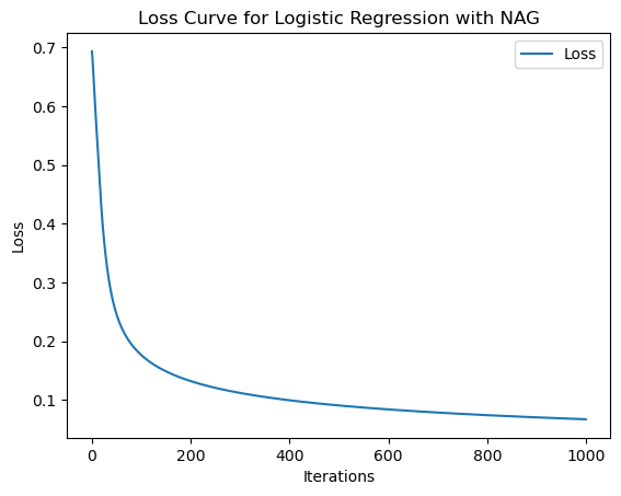
# 绘制损失曲线
plt.figure()
plt.plot(range(self.n_iters), losses, label="Loss")
plt.title("Loss Curve for Logistic Regression with NAG")
plt.xlabel("Iterations")
plt.ylabel("Loss")
plt.legend()
plt.show()
def predict(self, X):
linear_model = np.dot(X, self.weights) + self.bias
y_pred = self.sigmoid(linear_model)
return np.where(y_pred > 0.5, 1, 0)
# 生成数据
np.random.seed(0)
X = 2 * np.random.rand(100, 1)
y = (X > 1).astype(int).ravel() # 生成二分类标签
# 训练模型
model = LogisticRegressionNAG(learning_rate=0.1, momentum=0.9, n_iters=1000)
model.fit(X, y)
# 预测
X_new = np.array([[0], [2]])
y_pred = model.predict(X_new)
# 绘制预测结果
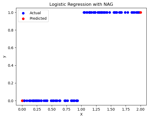
plt.figure()
plt.scatter(X, y, color='blue', label="Actual")
plt.scatter(X_new, y_pred, color='red', label="Predicted")
plt.title("Logistic Regression with NAG")
plt.xlabel("X")
plt.ylabel("y")
plt.legend()
plt.show()不同迭代次数下的模型损失loss
经过NAG优化后的模型的预测效果(红点)
Adaptive Gradient, AdaGrad
对于之前讨论的所有算法,学习率都是固定的。
Adaptive Gradient(AdaGrad)算法是一种自适应学习率的优化算法,于2011年由Duchi等人提出,它能够根据参数的历史梯度自适应地调整学习率。
核心思想
AdaGrad的核心思想是对每个参数的学习率进行适应性调整,从而实现对参数的不同历史梯度的平方和进行自适应调整。
具体来说,AdaGrad通过累积过去所有梯度的平方和来为每个参数动态调整学习率,使得较少更新频繁出现的特征参数具有更大的学习率,而较频繁更新的特征参数则具有更小的学习率。
数学原理
- 梯度计算: $$ g = \nabla{\theta{k-1}} L(\theta) $$ 计算损失函数 $ L(\theta)$ 关于参数 $\theta $ 在第 $k-1$ 次迭代时的梯度 $g $ ;其中$\nabla{\theta}$表示梯度运算符,$\theta{k-1}$表示上一步的参数值。
- 累积梯度平方和更新:
$$
rk = r{k-1} + g \odot g
$$
在第 k 次迭代时,将当前梯度 g 的平方(逐元素相乘)累加到之前的累积梯度平方和 $ r_{k-1} $ 上,得到新的累积梯度平方和 $ r_k $ 。其中,$\odot$表示元素乘法(即Hadamard乘积)。
- 自适应学习率计算: $$ \eta = \frac{\eta_0}{\sqrt{r_k + \epsilon}} $$ 计算自适应学习率,其中 $ \eta_0 $ 是初始学习率, $ r_k $ 是当前的累积梯度平方和, $ \epsilon $ 是一个小的正数(防止除零错误)。通过累积梯度平方和$r_k$来调整学习率$\epsilon$;这样的调整使得学习率对于出现频繁的特征会更小,而对于稀疏特征会更大,有助于提高模型在稀疏数据上的性能
- 参数更新: $$ \theta_k = \theta - \eta g $$
完整形式:
$$
\thetak = \theta - \frac{\eta_0}{\sqrt{r_k + \epsilon}} * \nabla{\theta_{k-1}} L(\theta)
$$
使用计算出的自适应学习率 $ \eta $ 和梯度 $ g $ 来更新参数 $ \theta $ 到新值 $ \theta_k $ ,目的是减少损失函数 $ L(\theta) $ 的值。
优缺点
Advantage: 不需要手动更新学习率
Disadvantage:
- 学习率持续衰减:由于累积的平方梯度持续增加,学习率会持续衰减,最终导致学习率过小,从而使得训练后期模型难以收敛。
- 存储梯度平方和:需要为每个参数存储一个累积的梯度平方和,这在参数很多时会增加额外的内存开销。
案例
以下是一个基于Adaptive Gradient(AdaGrad)优化算法的Python代码示例,并附带了优化过程的可视化效果。我们将使用一个简单的二维函数 $f(x)=x_1^2+x_2^2$ 来展示优化过程,并通过Matplotlib绘制优化路径。
import numpy as np
import matplotlib.pyplot as plt

# 定义目标函数
def f(x):
    return x[0]**2 + x[1]**2  # 示例函数:f(x) = x1^2 + x2^2

# 定义目标函数的梯度
def grad_f(x):
    return np.array([2*x[0], 2*x[1]])  # 示例函数的梯度

# AdaGrad优化算法
def Adagrad(x_init, step_size, n_iters):
    eta = step_size
    G_t = 0  # 累积梯度的平方
    eps = 1e-8  # 防止分母为零的小常数
    theta = np.tile(x_init, (n_iters, 1))  # 初始化参数
    z = np.tile([f(x_init)], n_iters)  # 初始化目标函数值

    for k in range(1, n_iters):
        # 计算梯度
        g_t = grad_f(theta[k-1])
        # 累积梯度的平方
        G_t += g_t**2
        # 更新参数
        theta[k] = theta[k-1] - eta * g_t / (np.sqrt(G_t) + eps)
        # 计算目标函数值
        z[k] = f(theta[k])

    # 返回优化过程中的参数和目标函数值
    return theta, z

# 初始化参数
x_init = np.array([1.0, 1.0])  # 初始参数
step_size = 0.1  # 学习率
n_iters = 50  # 迭代次数

# 运行AdaGrad优化算法
theta, z = Adagrad(x_init, step_size, n_iters)

# 可视化优化过程
# 绘制目标函数的等高线图
x1 = np.linspace(-2, 2, 400)
x2 = np.linspace(-2, 2, 400)
X1, X2 = np.meshgrid(x1, x2)
Z = X1**2 + X2**2

plt.figure(figsize=(10, 6))
contour = plt.contour(X1, X2, Z, levels=50, cmap='viridis')
plt.clabel(contour, inline=True, fontsize=8)
plt.title("AdaGrad Optimization Path")
plt.xlabel("x1")
plt.ylabel("x2")

# 绘制优化路径
plt.plot(theta[:, 0], theta[:, 1], 'r-', linewidth=2, label="AdaGrad Path")
plt.scatter(theta[:, 0], theta[:, 1], c='r', s=50, zorder=5)
plt.scatter([0], [0], c='g', s=100, label="Global Minimum")

plt.legend()
plt.show()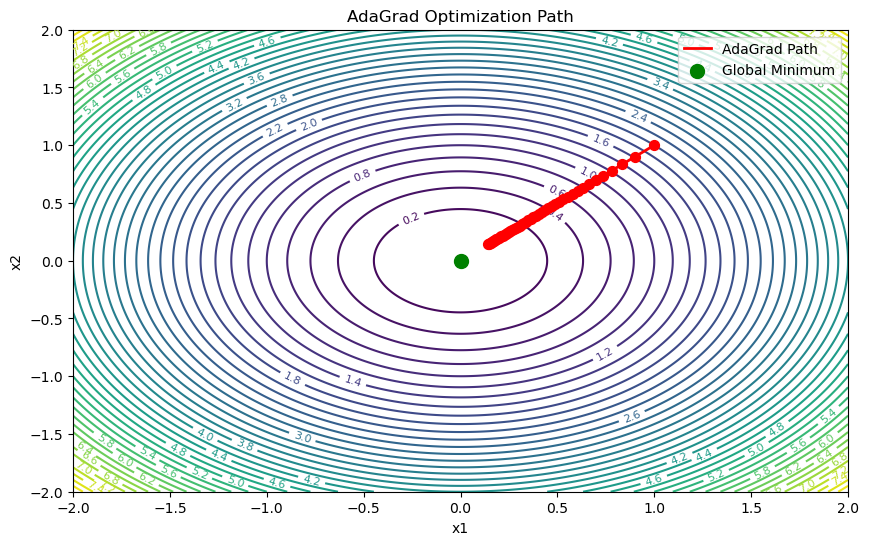
AdaDelta
基本原理
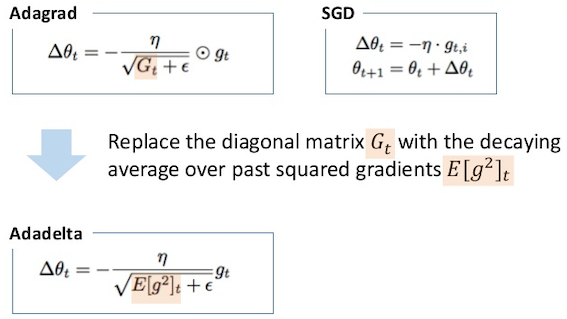
AdaGrad存在的问题是,随着迭代次数的增加,学习率会变得非常小,这导致收敛速度变慢。为了避免这个问题,AdaDelta算法采用了一种想法,即取梯度的指数衰减平均值。
AdaDelta是Adagrad的一个更稳健的扩展,它根据梯度更新的移动窗口来调整学习率,而不是累积所有过去的梯度。这样,即使进行了很多次更新,AdaDelta也能够继续学习。
AdaDelta算法并没有低效地存储过去的平方梯度,而是将梯度的累积和递归地定义为所有过去平方梯度的衰减平均值。
在时间步 $t$ 的运行平均$Eg^2_t$仅依赖于先前的累积平均值和当前的梯度:
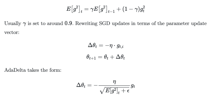
在AdaDelta算法中不需要设置默认的学习率:
优缺点
Advantage:
- AdaDelta不需要手动设置学习率,因为它会根据迭代过程中的梯度信息来自适应地调整学习率。
- 对稀疏数据表现良好:在处理稀疏数据时,AdaDelta能够动态调整学习率,防止学习率过快减小,从而避免收敛速度变慢的问题。
- 减少对初始条件的敏感性:AdaDelta对初始化条件的敏感性较低,因为它会根据训练过程中的情况进行自适应调整。
Disadvantage:
收敛速度:与一些更新的优化方法(如Adam)相比,AdaDelta可能不会那么快地收敛。
案例
对经典的Rosenbrock函数进行优化:
$$f(x,y)=(1-x)^2+100(y-x^2)^2$$
这个函数只有一个全部最小值点$f(x,y)=(1,1)$,并且在 $(0,0) $附近有一个较深的山谷
import numpy as np
import matplotlib.pyplot as plt

# 定义Rosenbrock函数
def f(x):
    return (1 - x[0])**2 + 100 * (x[1] - x[0]**2)**2

# 定义Rosenbrock函数的梯度
def grad_f(x):
    return np.array([
        -2 * (1 - x[0]) - 400 * x[0] * (x[1] - x[0]**2),
        200 * (x[1] - x[0]**2)
    ])

# AdaDelta优化算法
def adadelta_optimizer(x_init, num_iter=100, rho=0.9, epsilon=1e-8):
    """
    x_init: 初始参数
    num_iter: 迭代次数
    rho: 衰减率
    epsilon: 无穷小量
    """
    # 初始化参数
    x = x_init
    E_g2 = np.zeros_like(x)  # 梯度平方的指数加权移动平均
    E_delta_x2 = np.zeros_like(x)  # 参数更新量平方的指数加权移动平均
    x_history = [x.copy()]  # 保存优化路径
    f_history = [f(x)]  # 保存目标函数值

    for i in range(num_iter):
        # 计算梯度
        g = grad_f(x)
        # 更新梯度平方的指数加权移动平均
        E_g2 = rho * E_g2 + (1 - rho) * g**2
        # 计算参数更新量
        delta_x = -np.sqrt(E_delta_x2 + epsilon) / np.sqrt(E_g2 + epsilon) * g
        # 更新参数
        x += delta_x
        # 更新参数更新量平方的指数加权移动平均
        E_delta_x2 = rho * E_delta_x2 + (1 - rho) * delta_x**2
        # 保存优化路径和目标函数值
        x_history.append(x.copy())
        f_history.append(f(x))

    return np.array(x_history), np.array(f_history)

# 初始化参数
x_init = np.array([-1.5, 1.5])  # 初始参数
num_iter = 100  # 迭代次数

# 运行AdaDelta优化算法
x_history, f_history = adadelta_optimizer(x_init, num_iter=num_iter)

# 可视化优化过程
# 绘制Rosenbrock函数的等高线图
x1 = np.linspace(-2, 2, 400)
x2 = np.linspace(-1, 3, 400)
X1, X2 = np.meshgrid(x1, x2)
Z = (1 - X1)**2 + 100 * (X2 - X1**2)**2

plt.figure(figsize=(10, 6))
contour = plt.contour(X1, X2, Z, levels=50, cmap='viridis')
plt.clabel(contour, inline=True, fontsize=8)
plt.title("AdaDelta Optimization Path for Rosenbrock Function")
plt.xlabel("x1")
plt.ylabel("x2")

# 绘制优化路径
plt.plot(x_history[:, 0], x_history[:, 1], 'r-', linewidth=2, label="AdaDelta Path")
plt.scatter(x_history[:, 0], x_history[:, 1], c='r', s=50, zorder=5)
plt.scatter([1], [1], c='g', s=100, label="Global Minimum")

plt.legend()
plt.show()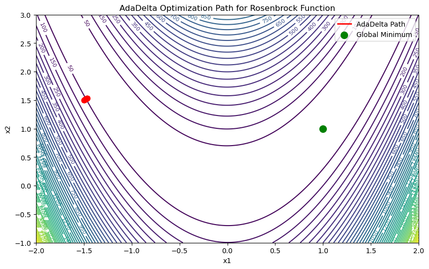
RMSprop(Root Mean Square Propagation)
基本原理
RMSprop(Root Mean Square Propagation)算法是一种自适应学习率的优化算法,由 Geoffrey Hinton 提出,旨在解决梯度下降及其变体在优化过程中学习率固定不变时可能导致的收敛速度慢或不收敛的问题。
RMSprop通过为每个参数动态调整学习率来改进这一点,特别适用于处理非平稳目标函数。
基本原理:
- 初始化:
- 参数$\theta$
- 梯度平方的指数加权平均值$Eg^2$为0
- 设置学习率$ η $(比如0.001)
- 设置衰减率 ρ(比如0.9)
- 梯度计算
在每次迭代中,计算损失函数 $L(θ)$关于参数$θ$的梯度$g$
- 更新梯度平方的指数加权平均值$Eg^2$:
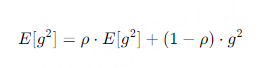
- 参数更新
使用下面的参数更新参数$\theta$
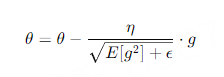
其中,$ϵ$ 是一个小的正数(例如$10^{−8}$),用于防止除零错误。
优缺点
Advantage:
- 自适应学习率:RMSprop为每个参数动态调整学习率,使得学习率与梯度的平方的指数加权平均值的平方根成反比。这有助于处理稀疏数据和非平稳目标函数。
- 防止梯度爆炸:通过限制梯度更新的幅度,RMSprop有助于防止梯度爆炸问题。
- 无需手动调整学习率:RMSprop自动调整学习率,减少了手动调整学习率的需求。
Disadvantage:
- 可能需要调整超参数:尽管RMSprop自动调整学习率,但仍然需要选择合适的衰减率 ρ 和学习率 η。
- 在某些情况下可能不稳定:在某些情况下,RMSprop可能不如其他优化算法(如Adam)稳定。
案例
import numpy as np
import matplotlib.pyplot as plt

# 定义Himmelblau函数
def f(x):
    return (x[0]**2 + x[1] - 11)**2 + (x[0] + x[1]**2 - 7)**2

# 定义Himmelblau函数的梯度
def grad_f(x):
    return np.array([
        4 * x[0] * (x[0]**2 + x[1] - 11) + 2 * (x[0] + x[1]**2 - 7),
        2 * (x[0]**2 + x[1] - 11) + 4 * x[1] * (x[0] + x[1]**2 - 7)
    ])

# RMSprop优化算法
def rmsprop_optimizer(x_init, num_iter=100, learning_rate=0.001, rho=0.9, epsilon=1e-8):
    """
    x_init: 初始参数
    num_iter: 迭代次数
    learning_rate: 学习率
    rho: 衰减率
    epsilon: 无穷小量
    """
    # 初始化参数
    x = x_init
    v = np.zeros_like(x)  # 梯度平方的累积
    x_history = [x.copy()]  # 保存优化路径
    f_history = [f(x)]  # 保存目标函数值

    for i in range(num_iter):
        # 计算梯度
        g = grad_f(x)
        # 更新梯度平方的累积
        v = rho * v + (1 - rho) * g**2
        # 更新参数
        x -= learning_rate * g / (np.sqrt(v) + epsilon)
        # 保存优化路径和目标函数值
        x_history.append(x.copy())
        f_history.append(f(x))

    return np.array(x_history), np.array(f_history)

# 初始化参数
x_init = np.array([0.0, 0.0])  # 初始参数
num_iter = 100  # 迭代次数

# 运行RMSprop优化算法
x_history, f_history = rmsprop_optimizer(x_init, num_iter=num_iter)

# 可视化优化过程
# 绘制Himmelblau函数的等高线图
x1 = np.linspace(-5, 5, 400)
x2 = np.linspace(-5, 5, 400)
X1, X2 = np.meshgrid(x1, x2)
Z = (X1**2 + X2 - 11)**2 + (X1 + X2**2 - 7)**2

plt.figure(figsize=(10, 6))
contour = plt.contour(X1, X2, Z, levels=50, cmap='viridis')
plt.clabel(contour, inline=True, fontsize=8)
plt.title("RMSprop Optimization Path for Himmelblau Function")
plt.xlabel("x1")
plt.ylabel("x2")

# 绘制优化路径
plt.plot(x_history[:, 0], x_history[:, 1], 'r-', linewidth=2, label="RMSprop Path")
plt.scatter(x_history[:, 0], x_history[:, 1], c='r', s=50, zorder=5)
plt.scatter([3], [2], c='g', s=100, label="Global Minimum")
plt.scatter([-2.8051, -3.7793, 3.5844], [3.1313, -3.2832, -1.8481], c='b', s=100, label="Local Minima")

plt.legend()
plt.show()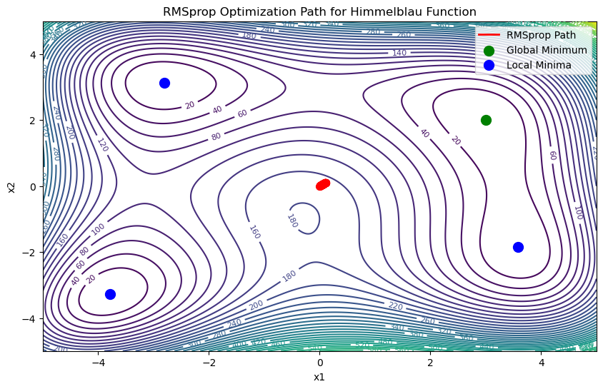
优化器9:Adaptive Moment Estimation(Adam)
在机器学习中,Adam(Adaptive Moment Estimation,自适应矩估计)作为一种高效的优化算法脱颖而出。它旨在调整每个参数的学习率。
基本原理
Adam可以看作是结合了RMSprop和带动量的随机梯度下降(SGD with Momentum)的优化算法。
Adam为每个参数计算自适应学习率。除了像AdaDelta和RMSprop那样存储过去梯度平方的指数衰减平均值$v_t$之外,Adam还维护了一个过去梯度的指数衰减平均值$m_t$,这与动量方法类似。
如果说动量可以被看作是一个在斜坡上滚动的球,那么Adam的行为则像是一个带有摩擦的重球,因此它更倾向于在误差曲面的平坦最小值处停留。
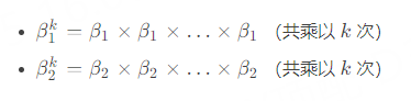
数学公式
核心:Adam通过考虑梯度的一阶矩和二阶矩的移动平均值,改进了梯度下降的方法,使得它能够智能地适应每个参数的学习率。
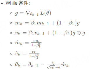
其中,$m_k和v_k$分别是梯度的一阶矩和二阶矩的估计,$\beta_1和\beta_2$是控制两个矩估计得指数衰减率,范围在0到1之间,通常设置为0.9和0.999。$\epsilon$是个非常小的数(例如1e-8),防止除数为零。k是当前迭代的次数,用于做偏差校正。
Adam代码的核心代码:
def adam_update(parameters, gradients, m, v, t, lr=0.001, beta1=0.9, beta2=0.999, epsilon=1e-8):
    for param, grad in zip(parameters, gradients):
        m[param] = beta1 * m[param] + (1 - beta1) * grad
        v[param] = beta2 * v[param] + (1 - beta2) * (grad ** 2)
        m_corrected = m[param] / (1 - beta1 ** t)
        v_corrected = v[param] / (1 - beta2 ** t)
        param_update = lr * m_corrected / (np.sqrt(v_corrected) + epsilon)
        param -= param_update
案例
import numpy as np
import matplotlib.pyplot as plt

# 目标函数
def func(X):
    return 5 * X[0, 0]**2 + 2 * X[1, 0]**2 + 3 * X[0, 0] - 10 * X[1, 0] + 4

# 目标函数的梯度
def grad(X):
    grad_x1 = 10 * X[0, 0] + 3
    grad_x2 = 4 * X[1, 0] - 10
    return np.array([[grad_x1], [grad_x2]])

# Adam优化器类
class Adam:
    def __init__(self, func, grad, seed):
        self.func = func
        self.grad = grad
        self.seed = seed
        self.xPath = []
        self.JPath = []

    def get_solu(self, alpha=0.001, beta1=0.9, beta2=0.999, epsilon=1e-8, zeta=1e-6, maxIter=1000):
        self.xPath = []
        self.JPath = []
        x = self.seed
        JVal = self.func(x)
        self.xPath.append(x)
        self.JPath.append(JVal)
        grad = self.grad(x)
        m, v = np.zeros(x.shape), np.zeros(x.shape)
        for k in range(1, maxIter + 1):
            m = beta1 * m + (1 - beta1) * grad
            v = beta2 * v + (1 - beta2) * (grad ** 2)
            m_hat = m / (1 - beta1 ** k)
            v_hat = v / (1 - beta2 ** k)
            x = x - alpha * m_hat / (np.sqrt(v_hat) + epsilon)
            JVal = self.func(x)
            self.xPath.append(x)
            self.JPath.append(JVal)
            grad = self.grad(x)
            if np.linalg.norm(grad) < zeta:
                break
        return x, JVal

# 可视化类
class AdamPlot:
    @staticmethod
    def plot_fig(adamObj):
        x, JVal = adamObj.get_solu(alpha=0.1)
        xPath = np.array(adamObj.xPath)
        JPath = adamObj.JPath
        fig = plt.figure(figsize=(12, 6))
        ax1 = plt.subplot(1, 2, 1)
        ax2 = plt.subplot(1, 2, 2)

        # 绘制损失值变化
        ax1.plot(JPath, "k.", markersize=5)
        ax1.plot(0, JPath[0], "go", label="Starting Point")
        ax1.plot(len(JPath) - 1, JPath[-1], "r*", label="Solution")
        ax1.set_xlabel("Iteration")
        ax1.set_ylabel("Loss")
        ax1.legend()

        # 绘制优化路径
        x1 = np.linspace(-10, 10, 300)
        x2 = np.linspace(-10, 10, 300)
        x1, x2 = np.meshgrid(x1, x2)
        f = 5 * x1**2 + 2 * x2**2 + 3 * x1 - 10 * x2 + 4
        ax2.contour(x1, x2, f, levels=50)
        ax2.plot(xPath[:, 0, 0], xPath[:, 1, 0], "k--", lw=2)
        ax2.plot(xPath[0, 0, 0], xPath[0, 1, 0], "go", label="Starting Point")
        ax2.plot(xPath[-1, 0, 0], xPath[-1, 1, 0], "r*", label="Solution")
        ax2.set_xlabel("$x_1$")
        ax2.set_ylabel("$x_2$")
        ax2.legend()

        plt.tight_layout()
        plt.show()

# 主程序
if __name__ == "__main__":
    seed = np.array([[1.0], [1.0]])  # 初始点
    adamObj = Adam(func, grad, seed)
    AdamPlot.plot_fig(adamObj)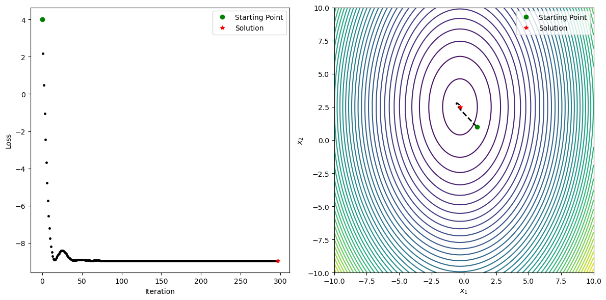
参考
1、https://www.kdnuggets.com/2020/12/optimization-algorithms-neural-networks.html
2、https://blog.csdn.net/qq_38156104/article/details/106739700
3、https://medium.com/@piyushkashyap045/understanding-nesterov-accelerated-gradient-nag-340c53d64597
4、https://blog.csdn.net/m0_48923489/article/details/136854257
5、https://blog.csdn.net/m0_48923489/article/details/136863726
6、Adam: A Method for Stochastic Optimization
Diederik P. Kingma, Jimmy Ba
原创声明:本文系作者授权腾讯云开发者社区发表,未经许可,不得转载。
如有侵权,请联系 cloudcommunity@tencent.com 删除。
原创声明:本文系作者授权腾讯云开发者社区发表,未经许可,不得转载。
如有侵权,请联系 cloudcommunity@tencent.com 删除。
评论
登录后参与评论
推荐阅读
目录
腾讯云开发者

Copyright © 2013 - 2026 Tencent Cloud. All Rights Reserved. 腾讯云 版权所有
深圳市腾讯计算机系统有限公司 ICP备案/许可证号:粤B2-20090059 ![]() 粤公网安备44030502008569号
粤公网安备44030502008569号
腾讯云计算(北京)有限责任公司 京ICP证150476号 | 京ICP备11018762号