R tips：使用最近邻算法进行空间浸润带的计算

本文使用最近邻算法进行浸润带的计算。

空间组学中，有的时候需要对免疫浸润带进行特定距离的划分，形成一层一层的浸润区域。

以10X的官方xenium示例数据为例https://www.10xgenomics.com/datasets/ffpe-human-breast-with-pre-designed-panel-1-standard。

圈选ROI并计算浸润边界

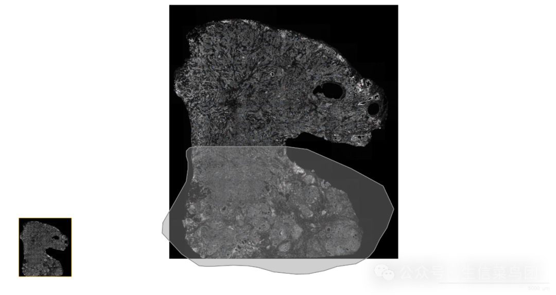
下载的数据使用Xenium explorer打开，然后找到需要进行计算浸润带的位置，并根据方向将相应的全部选中。

如下图所示，假设中间的位置是需要进行浸润带计算的位置，而需要计算浸润带的方向是向下，则在Xenium explorer中选择套索工具仔细的圈画浸润边界，并将浸润带计算方向上的所有细胞选中。

然后在Xenium explorer中将图示的ROI区域的边界坐标下载下来。

由于Xenium explorer无法圈画单条线，至少也是一个闭合区域，因此需要先计算好浸润边界的位置：

1. library(tidyverse)
2. library(sp)
4. # 读取ROI的边界坐标及细胞的质心坐标
5. tumor_boundary <- read_csv("data/coordinates.csv", skip = 2)
6. cells_position <- arrow::read_parquet("Xenium_V1_FFPE_Human_Breast_IDC/cells.parquet")
8. # 然后根据ROI边界坐标，将细胞分配到ROI中
9. cell_idx <-
10. sp::point.in.polygon(
11. cells_position$x_centroid, # point
12. cells_position$y_centroid, # point
13. tumor_boundary$X, # polygon
14. tumor_boundary$Y
15. ) %>%
16. as.logical # only 0 is FALSE, all others is TRUE
18. # 于是tumor_area_1即是ROI中的细胞，图示中的所有细胞
19. # tumor_area_2是剩余细胞，也就是图示中的上方未被框选中的细胞
20. tumor_area_1 <- cells_position[cell_idx, ] %>% mutate(x = x_centroid, y = y_centroid )
21. tumor_area_2 <- cells_position[!cell_idx, ] %>% mutate(x = x_centroid, y = y_centroid )

获得了浸润边界的两组细胞之后，就可以进行浸润边界的计算：

1. # 根据tumor_area_1和tumor_area_2找到绘制的tumor boundary
2. # 寻找1和2中的最近邻点，以20um（大概一个细胞，根据效果调整）为限度，
3. # 如果没有nn点则不是边界点。
4. # 找到1和2中的边界点，取均值即是最终的边界点
6. # dat: tumor_area_1
7. # query: tumor_area_2
8. nn_left_right <-
9. RANN::nn2(
10. tumor_area_1[2:3],
11. tumor_area_2[2:3],
12. k = 10,
13. searchtype = 'radius',
14. radius = 20 # 若边界未能找到，则调整radius的值
15. )
17. non_boundary_idx <- apply(nn_left_right$nn.idx == 0, 1, all)
18. if(sum(non_boundary_idx) == nrow(tumor_area_2)){
19. print("radius is small, no boundary point.")
20. }
22. boundary_idx_1 <- nn_left_right$nn.idx[! non_boundary_idx, 1]
23. boundary_1 <- tumor_area_1[boundary_idx_1, ]
24. boundary_idx_2 <- ! non_boundary_idx
25. boundary_2 <- tumor_area_2[boundary_idx_2, ]
28. # comuted boudary coords
29. boundary_coords_df <-
30. data.frame(
31. x = (boundary_1x_centroid + boundary_2x_centroid) / 2,
32. y = (boundary_1y_centroid + boundary_2y_centroid) / 2
33. )

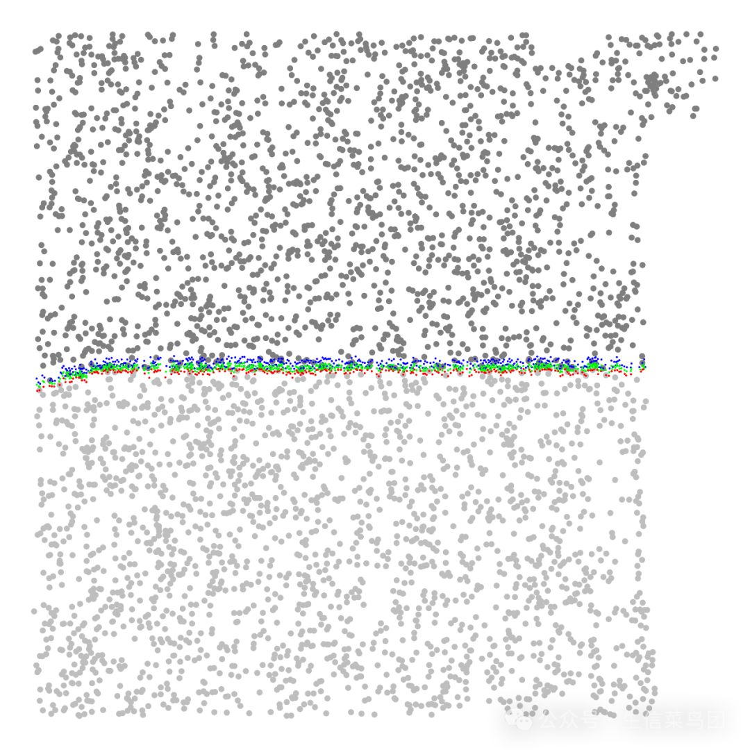
绘图展示，计算的圈画的浸润边界位置：

1. # 只展示浸润边界附近区域的细胞
2. boundary_df_for_plot <-
3. boundary_coords_df %>%
4. .[chull(.), ] %>%
5. map(range) %>%
6. map(~ .x + c(-500, 500))
8. # 定义用于筛选细胞的函数
9. filter_points <- function(dat, boundary){
10. x_idx <- datx_centroid < boundary
11. y_idx <- daty_centroid < boundary
13. dat[x_idx & y_idx, ]
14. }
16. # 绘图
17. ggplot() +
18. geom_point(
19. # left area
20. data = tumor_area_1 %>% dplyr::slice_sample(prop = 0.1) %>% filter_points(boundary_df_for_plot), # 仅绘制10%的点，加快绘制速度
21. aes(x = x_centroid, y = -y_centroid),
22. color = "gray"
23. ) +
24. geom_point(
25. # right area
26. data = tumor_area_2 %>% dplyr::slice_sample(prop = 0.1) %>% filter_points(boundary_df_for_plot), # 仅绘制10%的点，加快绘制速度
27. aes(x = x_centroid, y = -y_centroid),
28. color = "gray50"
29. ) +
31. geom_point(
32. # comute left_boundary
33. data = boundary_1,
34. aes(x = x, y = -y),
35. color = "red",
36. size = 0.1
37. ) +
38. geom_point(
39. # compute right_boundary
40. data = boundary_2,
41. aes(x = x, y = -y),
42. color = "blue",
43. size = 0.1
44. ) +
45. geom_point(
46. # the final tumor boundary
47. data = boundary_coords_df,
48. aes(x = x, y = -y),
49. color = "green",
50. size = 0.1
51. ) +
52. theme_void()

如下图所示，计算的浸润边界是绿色点，用于计算浸润边界的上下边界配对点是红蓝色点。

使用最近邻算法往下寻找浸润区域

假设需要以250um为单位，分别找到250um 500um及750um的浸润区域，则可如下操作：

先定义一个最近邻的工具函数：

1. # reduceFindNN find all (k) nn points in a certain radius,
2. # k would be increased when k is not enough for a certain radius
3. reduceFindNN <- function(dat, k = 10, query = NULL, searchtype = "radius", radius = 100, mpp = 1, max_k = 2000){
4. if(is.null(query)){
5. query <- dat
6. }
8. stopifnot(all(c('x', 'y') %in% colnames(dat)))
9. stopifnot(all(c('x', 'y') %in% colnames(query)))
11. dat <- dat[c('x', 'y')]
12. query <- query[c('x', 'y')]
14. nn_dat <- RANN::nn2(
15. dat,
16. query = query,
17. k = k,
18. radius = radius / mpp # radius, um -> pixel
19. )
21. k_enough <- sum(apply(nn_dat
22. cat(str_glue("k is {k} and is enough for {k_enough * 100}% cells.\n\n"))
24. while(k < max_k && k_enough < 0.99){
26. if(k < 700){
27. k <- k + 100
28. }else if(k < 2000){
29. k <- k + 200
30. }else if(k < 5000){
31. k <- k + 500
32. }else{
33. k <- k + 1000
34. }
36. nn_dat <- RANN::nn2(
37. dat,
38. query = query,
39. searchtype = searchtype,
40. k = k,
41. radius = radius / mpp # radius, um -> pixel
42. )
44. k_enough <- sum(apply(nn_dat
45. cat(str_glue("k is {k} and is enough for {k_enough * 100}% cells.\n\n"))
47. }
48. return(nn_dat)
49. }

浸润带的计算：

1. radius_ls <- c(250, 500, 750) %>% set_names(., .)
3. coords_tumor_infiltration_ls <-
4. radius_ls %>%
5. map(function(radius){
6. dat_nn <-
7. reduceFindNN(
8. dat = tumor_area_1, # %>% rbind(tumor_boundary_coords) %>% distinct(),
9. query = boundary_coords_df, # tumor_boundary_coords,
10. radius = radius,
11. mpp = 1,
12. k = 100,
13. max_k = nrow(tumor_area_1) # 2000
14. )
17. # all nn points is infiltration points
18. points_idx <- dat_nn$nn.idx %>% c() %>% .[. != 0] %>% unique
20. # infiltration area
21. coords <- tumor_area_1[points_idx, ]
22. coords
23. })

750um浸润带减去500um浸润带就是500-750um浸润带，以此类推：

1. # 当前浸润带减去上一层的浸润带
2. coords_tumor_infiltration_ls2 <- list()
3. for(i in rev(seq_along(coords_tumor_infiltration_ls))){
4. name <- names(coords_tumor_infiltration_ls)[i]
5. if(i == 1){
6. coords_tumor_infiltration_ls2[[name]] <- coords_tumor_infiltration_ls[[1]]
7. return()
8. }
9. present_df <- coords_tumor_infiltration_ls[[i]]
10. next_df <- coords_tumor_infiltration_ls[[i-1]]
11. coords_tumor_infiltration_ls2[[name]] <- present_df[!present_df
12. }
14. # 获得浸润带 ----------
15. coords_tumor_infiltration_df <-
16. coords_tumor_infiltration_ls2 %>%
17. enframe(name = "radius") %>%
18. unnest(value)

获得浸润区域如下：

1. p_infile_full <-
2. cells_position %>%
3. ggplot(aes(x = x_centroid , y = -y_centroid)) +
4. geom_point() +
5. geom_point(
6. data = boundary_coords_df,
7. aes(x = x, y = -y),
8. color = "red",
9. size = 0.5
10. ) +
11. geom_point(
12. data = coords_tumor_infiltration_df,
13. aes(x = x, y = -y, color = radius),
14. # color = "blue",
15. alpha = 0.5,
16. size = 0.5
17. ) +
18. theme_void()
21. p_infile_subset <-
22. cells_position %>%
23. dplyr::slice_sample(prop = 0.1) %>%
24. filter_points(boundary_df_for_plot) %>%
25. ggplot(aes(x = x_centroid , y = -y_centroid)) +
26. geom_point() +
27. geom_point(
28. data = boundary_coords_df,
29. aes(x = x, y = -y),
30. color = "red",
31. size = 0.5
32. ) +
33. geom_point(
34. data = coords_tumor_infiltration_df,
35. aes(x = x, y = -y, color = radius),
36. # color = "blue",
37. alpha = 0.5,
38. size = 0.5
39. ) +
40. theme_void()

如下图所示，浸润边界的浸润带展示：

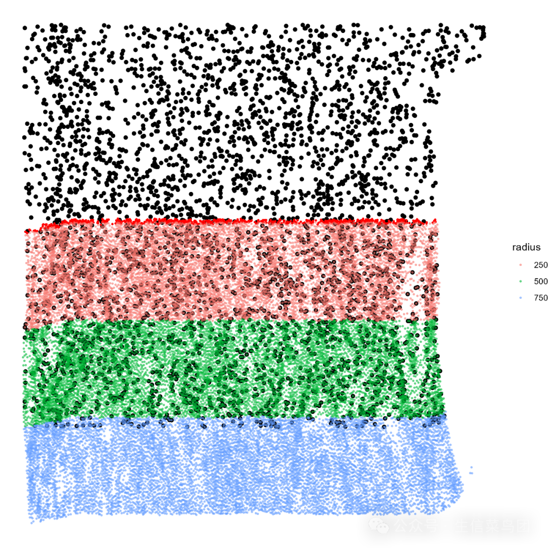
全图展示的浸润带：