圆柱形翅片(销鳍)的Simscape模型
圆柱形翅片(销鳍)的Simscape模型
提问于 2016-07-24 00:17:38
我想建立一个引脚鳍的热模型:

在圆柱体的左侧(红线),140°C的温度加热翅片。无论是在表面和右边的汽缸(蓝线),一个对流换热器正在冷却的翅片。在针内,存在热传导。
在这种情况下,可以在文献中找到销鳍T(x)长度上温度分布的解析解,例如这里 (公式18.12):
通过以下方式:
其中:
- h_conv =W/m平方公里的对流换热
- h_cond = W/mK中的导电传热
- S=针的表面积(以平方米为单位)
- A=销鳍的截面积,以平方米为单位
- T_amb =℃环境温度
- T_base =翅片左端的温度(以摄氏度计)
- T_x =位置x处销钉鳍的温度
我把所有的方程放到Matlab脚本中来评估杆长的温度分布:
% Variables
r = 0.01; % Radius of the pin fin in m
l = 0.2; % Length of the pin fin in m
h_conv = 500; % Convective heat transfer in W/m²K
h_cond = 500; % Conductive heat transfer in W/mK
T_base = 140; % Temperature on the left end of the fin tip in °C
T_amb = 40; % Ambient temperature in °C
n_elem = 20; % Number of division
x = [0:l/n_elem:l]'; % Vector of division, necessary for evaluation
A = r^2 * pi; % Cross sectional area of the pin fin in m²
S = 2 * pi * r * l; % Surface area of the pin in m²
% Analytical solution
beta = sqrt((h_conv*S)/(h_cond*A));
f = cosh(beta*(l-x))/cosh(beta*l);
temp = f*(T_base-T_amb)+T_amb;
% Plot of the temperature distribution
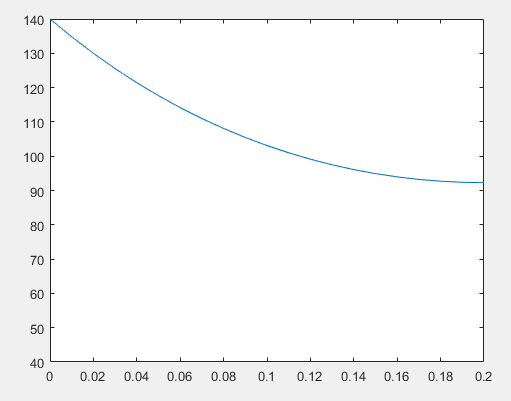
plot (x,temp);
axis([0 0.2 40 140]);产生的温度分布如下所示:
我尝试基于示例铁棒热传导构建该设置的Simscape模型。在解决了Simscape的问题之后,我对分析性解决方案和Simscape解决方案进行了比较:
x_ss     = [0:0.05:0.2]';                    % Vector of division, necessary for evaluation of the Simscape results
temp_ss  = [T_base,temp_simscape(end,:)]';   % Steady state results of Simscape model at 1/4, 2/4, 3/4 and 4/4 of the length

% Plot analytical vs. Simscape solution
plot (x,temp);
hold on;
plot (x_ss,temp_ss,'-o');
axis([0 0.2 40 140]);
分析和Simscape解决方案的对应图如下所示:
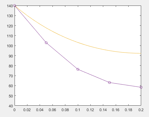
从图中可以看出,Simscape模型(蓝色曲线)预测的温度比解析解(橙色曲线)低得多。由于我无法找出这种差异的原因,我感谢任何帮助!
您可以下载模型这里。filehoster (www.xup.in)将模型的名称从"PinFin.mdl“转换为"PINFIN.MDL",因此需要将文件扩展名修改为".mdl”,以便在Matlab中打开它。
你好,菲尔
回答 1
Stack Overflow用户
发布于 2017-07-11 02:22:17
你用的是正确的方法。由于β参数的计算,结果不匹配。您有beta = sqrt((h_conv_S)/(h_cond_A));
尺寸是错误的,您需要: beta = sqrt((h_conv_P/(h_cond_A));
这里P= 2*pi*r。
有了这些修正,您会发现这两个输出(分析和模拟)都匹配得很好,足够精细的离散化(我使用了n_elem = 20)。
页面原文内容由Stack Overflow提供。腾讯云小微IT领域专用引擎提供翻译支持
原文链接:
https://stackoverflow.com/questions/38550050
复制相关文章
![倒立摆:Simulink建模[通俗易懂]](https://ask.qcloudimg.com/http-save/yehe-8223537/9e2706ce1d9b8c5b8f20bd299d6e8201.jpg)


点击加载更多
相似问题
Kurento:多个中翅片钳
整理错误的查询?翅片组
Modelica诉Simscape
MATLAB Simscape模型不输出扭矩或抛出错误
如何提高基于Simscape物理模型的仿真速度?
添加站长 进交流群
领取专属 10元无门槛券
AI混元助手 在线答疑

关注 腾讯云开发者公众号
洞察 腾讯核心技术
剖析业界实践案例

社区富文本编辑器全新改版!诚邀体验~
全新交互,全新视觉,新增快捷键、悬浮工具栏、高亮块等功能并同时优化现有功能,全面提升创作效率和体验
腾讯云开发者
